Download
1 / 104
1.04k likes | 1.17k Vues
Combining Photometric and Geometric Constraints. Yael Moses IDC, Herzliya. Joint work with Ilan Shimshoni and Michael Lindenbaum, the Technion. Problem 1:. Recover the 3D shape of a general smooth surface from a set of calibrated images. Problem 2:.

E N D
Combining Photometric and Geometric Constraints Yael Moses IDC, Herzliya Joint work with Ilan Shimshoni and Michael Lindenbaum, the Technion Y. Moses
Problem 1: • Recover the 3D shape of a general smooth surface from a set of calibrated images Y. Moses
Problem 2: Recover the 3D shape of a smooth bilaterally symmetric object from a single image. Y. Moses
Shape Recovery • Geometry: Stereo • Photometry: • Shape from shading • Photometric stereo Main problems: Calibrations and Correspondence Y. Moses
3D Shape Recovery Photometry: • Shape from shading • Photometric stereo Geometry: • Stereo • Structure from motion Y. Moses
Geometric Stereo • 2 different images • Known camera parameters • Known correspondence + + Y. Moses
Photometric Stereo • 3D shape recovery: surface normals from two or more images taken from the same viewpoint Y. Moses
Three images Photometric Stereo Solution: Matrix notation Y. Moses
Photometric Stereo Main Limitation: Correspondence is obtained by a fixed viewpoint • 3D shape recovery (surface normals) Two or more images taken from the same viewpoint Y. Moses
Overview • Combining photometric and geometric stereo: • Symmetric surface, single image • Non symmetric: 3 images • Mono-Geometric stereo • Mono-Photometric stereo • Experimental results. Y. Moses
The input • Smooth featureless surface • Taken under different viewpoints • Illuminated by different light sources • The Problem: • Recover the 3D shape from a set of calibrated images Y. Moses
n n * • Perspective projection Assumptions • Three or more images • Given correspondence the normals can be computed (e.g., Lambertian, distant point light source …) * Y. Moses
Our method Combines photometric and geometric stereo We make use of: • Given Correspondence: • Can compute a normal • Can compute the 3D point Y. Moses
Basic Method Given Correspondence Y. Moses
First Order Surface Approximation Y. Moses
First Order Surface Approximation Y. Moses
P() = (1 - )O1+ P, N(P() - P) = 0 First Order Surface Approximation Y. Moses
First Order Surface Approximation Y. Moses
New Correspondence Y. Moses
New Surface Approximation Y. Moses
Dense Correspondence Y. Moses
Basic Propagation Y. Moses
Basic Propagation Y. Moses
Basic method: First Order • Given correspondence pi and L Pand n • Given P andn T • Given P, T andMi a new correspondence qi Y. Moses
Extensions • Using more than three images • Propagation: • Using multi-neighbours • Smart propagation • Second error approximation • Error correction: • Based on local continuity • Other assumptions on the surface Y. Moses
Multi-neighbors Propagation Y. Moses
Smart Propagation Y. Moses
Second Order: a Sphere (P-P())(N+N)=0 N P() P N+N N Y. Moses
Second Order Approximation Y. Moses
Second Order Approximation Y. Moses
Using more than three images • Reduce noise of the photometric stereo • Avoid shadowed pixels • Detect “bad pixels” • Noise • Shadows • Violation of assumptions on the surface Y. Moses
Smart Propagation Y. Moses
Error correction The compatibility of the local 3D shape can be used to correct errors of: • Correspondence • Camera parameters • Illumination parameters Y. Moses
Score • Continuity: • Shape • Normals • Albedo • The consistency of 3D points locations and the computed normals: • General case: full triangulation • Local constraints Y. Moses
Extensions • Using more than three images • Propagation: • Using multi-neighbours • Smart propagation • Second error approximation • Error correction: • Based on local continuity • Other assumptions on the surface Y. Moses
Real Images • Camera calibration • Light calibration • Direction • Intensity • Ambient Y. Moses
5pp 5nn 5pn 3pp 3nn Y. Moses
Detected Correspondence Y. Moses
Error correction + multi-neighbord Multi-neighbors Basic scheme (3 images) Error correction no multi-neighbors Y. Moses
Synthetic Images New Images Y. Moses
Ground truth Basic scheme Multi-neighbors Error correction Sec a Y. Moses
Ground truth Basic scheme Multi-neighbors Error correction Sec b Y. Moses
Ground truth Basic scheme Multi-neighbors Error correction Sec c Y. Moses
Ground truth Basic scheme Multi-neighbors Error correction Sec d Ground truth Basic scheme Multi-neighbors approx. Error correction Y. Moses