Download

1 / 32
710 likes | 1.74k Vues
Arrays, Records and Pointers. Arrays, Records and Pointers. Data structures are classified as either linear or nonlinear. Normally arrays and linked lists fall into linear data structures. Trees and graphs are treated as nonlinear structures. Linear Arrays.

E N D
Arrays, Records and Pointers • Data structures are classified as either linear or nonlinear. • Normally arrays and linked lists fall into linear data structures. • Trees and graphs are treated as nonlinear structures.
Linear Arrays • A linear array is a list of a finite number n of homogeneous data elements. • The length of data elements of the array can be obtained by the following formula: • Length = UB – LB + 1 • UB is upper bound and LB is the lower bound.
Algorithm 4.1(Traversing a Linear Array) • Here LA is a linear array with lower bound LB and upper bond UB. This algorithm traverses LA applying an operation PROCESS to each element of LA. • 1. [Initialize counter] Set K := LB • 2. Repeat steps 3 and 4 while K ≤ UB • 3. [Visit element] Apply PROCESS to LA[K] • 4. [Increase counter] Set K := K + 1 • 5. [End of Step 2 loop]
Algorithm 4.2(Inserting into a Linear Array) • INSERT(LA, N, K, ITEM) • Here LA is a linear array with N elements and K is a positive integer such that K ≤ N. This algorithm inserts an element ITEM into the Kth position in LA.
Algorithm 4.2(Inserting into a Linear Array) • 1. [Initialize counter] Set J := N • 2. Repeat steps 3 and 4 while J ≥ K • [Move Jth element downward] • 3. Set LA[J+1] := LA[J] • 4.[Decrease counter] Set J := J – 1 • [End of Step 2 loop] • 5. [Insert element] Set LA[K] := ITEM • 6. [Reset N] Set N := N + 1 • 7. Exit
Algorithm 4.3(Deleting from a Linear Array) • DELETE(LA, N, K, ITEM) • Here LA is a linear array with N elements and K is a positive integer such that K ≤ N. this algorithm deletes the Kthelement from LA.
Algorithm 4.3(Deleting from a Linear Array) • 1. Set ITEM := LA[K] • 2. Repeat steps for J = K to N - 1 • [Move J + 1st element upward] • Set LA[J] := LA[J + 1] • [End of Step 2 loop] • 3. [Reset the number N of elements in LA] • Set N := N - 1 • 4. Exit
Sorting; Bubble Sort • Let A be a list of n numbers. Sorting A refers to the operation of rearranging the elements of A so they are in increasing order, i.e., so that • A[1] < A[2]<………A[N]
How Bubble sort works? • Suppose the list of numbers A[1], A[2],…..A[N] is in memory. • See page # 74 for detail.
Algorithm 4.4(Bubble Sort) • BUBBLE (DATA, N) • 1. Repeat steps 2 and 3 for K = 1 to N – 1 • 2. Set PTR := 1 • 3. Repeat while PTR ≤ N – K • (a) if DATA[PTR] > DATA[PTR + 1], then: • interchange DATA[PTR]and DATA[PTR + 1] • [End of if structure] • (b) Set PTR := PTR + 1 • [End of inner loop] • [End of outer loop] • 4. Exit
Complexity of Bubble Sort Algorithm • = O(n2)
Searching • Linear Search • In algorithm 2.4, we used the following while loop header: • Repeat while LOC ≤ N And DATA[LOC]≠ITEM • Alternatively, we can do this as the first step: • LOC = N + 1 • The purpose of this initial statement is to avoid repeatedly testing whether or not we have reached the end of the array DATA.
Algo 4.5(Linear Search) • LINEAR(DATA, N, ITEM, LOC) • Here DATA is a linear array with N elements and ITEM is a given item of information. This algorithm finds the location LOC of ITEM in DATA, or sets LOC: = 0 if the search is unsuccessful.
LINEAR(DATA, N, ITEM, LOC) • 1. [Insert ITEM at the end of DATA] • Set DATA[N + 1] = ITEM • 2. [Initialize counter] Set LOC: = 1 • 3. [Search for item] • Repeat while DATA[LOC] ≠ ITEM • Set LOC := LOC + 1 • [End of loop] • 4. [Successful?] If LOC = N + 1, then Set LOC:=0 • 5. Exit
Complexity of Linear Search Algorithm • Discuss it yourself (also see page # 77)
Binary Search • Data is sorted in increasing order. • Extremely efficient algorithm. • This algorithm works as follows: • During each stage of our algorithm, our search for ITEM is reduced to a segment of elements of DATA: • DATA[BEG], DATA[BEG + 1], DATA[BEG + 2]……DATA[END]
Binary Search • Note that the variables BEG and END denote the beginning and end locations of the segment under consideration. • Algorithm compares ITEM with the middle element DATA[MID] of the segment, where MID is obtained by: • MID = INT((BEG + END)/2) • If DATA[MID] = ITEM, then the search is successful and we set LOC := MID, otherwise, a new segment of DATA is obtained as follows:
Binary Search • (a) If ITEM < DATA[MID], then ITEM can appear only in the left half of the segment: DATA[BEG], DATA[BEG + 1], DATA[BEG + 2]……DATA[MID - 1] So we reset END := MID – 1 and begin searching again. • (b) If ITEM > DATA[MID], then ITEM can appear only in the right half of the segment: DATA[MID+1], DATA[MID + 2], ……DATA[END] So we reset BEG := MID + 1 and begin searching again.
Binary Search • If ITEM is not in the DATA, then eventually we obtain • END < BEG • This condition signals that the search is unsuccessful and in such a case we assign • LOC := NULL. • Here NULL is a value that lies outside the set of indices of DATA. (In most cases, we can choose NULL = 0)
Algorithm 4.6 (Binary Search) • BINARY (DATA, LB, UB, ITEM, LOC) • Here DATA is a sorted array with lower bound LB and upper bound UB, and ITEM is a given item of information. • The variables BEG, END and MID denote respectively the beginning, end and the middle locations of a segment of elements of DATA. This algorithm finds the location LOC of ITEM in DATA or sets LOC = NULL.
BINARY (DATA, LB, UB, ITEM, LOC) • 1. Set BEG = LB, END = UB and • MID = INT((BEG + END)/2) • 2. Repeat steps 3 and 4 while BEG ≤ END and DATA[MID] ≠ ITEM • 3. if ITEM < DATA[MID], then • Set END = MID – 1 • else • Set BEG = MID + 1 • [End of if structure]
BINARY (DATA, LB, UB, ITEM, LOC) • 4. Set MID = INT ((BEG + END)/2) • [End of step 2 loop] • 5. if DATA[MID] = ITEM, then: • Set LOC = MID • else • Set LOC = NULL • [End of if structure] • 6. Exit
BINARY (DATA, LB, UB, ITEM, LOC) • See example 4.9 • See yourself the complexity of the binary search algorithm.
Multidimensional Arrays • The arrays whose elements are accessed by more than one subscript are termed as multidimensional arrays. • Two-Dimensional array • A two dimensional m × n array A is a collection of m.n data elements such that each element is specified by a pair of integers (such as J, K) called subscripts, with the property that
Multidimensional Arrays • 1 ≤ J ≤ m and 1 ≤ K ≤ m • The element of A with first subscript j and second subscript k will be denoted by • A[J, K]
Representation of Two-Dimensional Arrays in Memory • Let A be a two-dimensional m × n array. • Although A is pictured as a rectangular array of elements with m rows and n columns, the array will be represented in memory by a block of m.n sequential memory locations. • The programming language stores the array A • either (1) column by column, or what is called column-major order
Representation of Two-Dimensional Arrays in Memory • Or (2) row by row, in row major order. See fig 4.10 • For a linear array LA, the computer does not keep track of the address LOC(LA[K]) of every element LA[K] of LA, but does keep track of Base(LA), the address of first element of LA. The computer uses the formula: LOC (LA[K]) = Base(LA) + w(K - 1) to find address of LA[K].
Representation of Two-Dimensional Arrays in Memory • Here w is the number of words per memory cell for the array LA, and 1 is the lower bound of the index set of LA. • For Column-major order • LOC(A[J, K]) = Base(A) + w[M(K-1) + (J-1)] • For Row-major order • LOC(A[J, K]) = Base(A) + w[N(J-1) + (K-1)] • See example 4.12
Algorithm 4.7 (Matrix Multiplication) • MATMUL(A, B, C, M, P, N) • Let A be an M × P matrix array, and let B be a P × N matrix array. This algorithm stores the product of A and B in an M × N matrix array C.
MATMUL(A, B, C, M, P, N) • 1. Repeat steps 2 to 4 for I = 1 to M: • 2. Repeat steps 3 and 4 for J = 1 to N: • 3. Set C[I, J] = 0 • 4. Repeat for K = 1 to P: • C[I, J] = C[I, J] + A[I, K] * B[K, J] • [End of inner loop] • [End of step 2 middle loop] • [End of step 1 outer loop] • 5. Exit
SPARSE MATRICES • Matrices with relatively high proportion of zero entries are called sparse matrices.