Download
1 / 107
1.09k likes | 1.41k Vues
A Guided Tour of Finite Mixture Models: From Pearson to the Web ICML ‘01 Keynote Talk Williams College, MA June 29th 2001. Padhraic Smyth Information and Computer Science University of California, Irvine www.datalab.uci.edu. Outline. What are mixture models? Definitions and examples

E N D
A Guided Tour of Finite Mixture Models: From Pearson to the WebICML ‘01 Keynote TalkWilliams College, MAJune 29th 2001 Padhraic Smyth Information and Computer Science University of California, Irvine www.datalab.uci.edu
Outline • What are mixture models? • Definitions and examples • How can we learn mixture models? • A brief history and illustration • What are mixture models useful for? • Applications in Web and transaction data • Recent research in mixtures?
Acknowledgements • Students: • Igor Cadez, Scott Gaffney, Xianping Ge, Dima Pavlov • Collaborators • David Heckerman, Chris Meek, Heikki Mannila, Christine McLaren, Geoff McLachlan, David Wolpert • Funding • NSF, NIH, NIST, KLA-Tencor, UCI Cancer Center, Microsoft Research, IBM Research, HNC Software.
Finite Mixture Models Weightk ComponentModelk Parametersk
Example: Mixture of Gaussians • Gaussian mixtures:
Example: Mixture of Gaussians • Gaussian mixtures: Each mixture component is a multidimensional Gaussian with its own mean mkand covariance “shape” Sk
Example: Mixture of Gaussians • Gaussian mixtures: Each mixture component is a multidimensional Gaussian with its own mean mkand covariance “shape” Sk e.g., K=2, 1-dim: {q, a} = {m1, s1 , m2, s2 , a1}
Example: Mixture of Naïve Bayes Conditional Independence model for each component (often quite useful to first-order)
Mixtures of Naïve Bayes Terms 1 1 1 1 1 1 1 1 1 1 1 1 1 1 1 1 1 Documents 1 1 1 1 1 1 1 1 1 1 1 1 1 1 1 1 1 1 1 1 1 1 1 1 1 1
Mixtures of Naïve Bayes Terms 1 1 1 1 1 1 1 1 1 1 1 1 Component 1 1 1 1 1 1 1 Documents 1 1 1 1 1 1 1 1 1 1 1 1 1 1 1 Component 2 1 1 1 1 1 1 1 1 1 1 1 1 1 1
Other Component Models • Mixtures of Rectangles • Pelleg and Moore (ICML, 2001) • Mixtures of Trees • Meila and Jordan (2000) • Mixtures of Curves • Quandt and Ramsey (1978) • Mixtures of Sequences • Poulsen (1990)
Interpretation of Mixtures 1. C has a direct (physical) interpretation e.g., C = {age of fish}, C = {male, female}
Interpretation of Mixtures 1. C has a direct (physical) interpretation e.g., C = {age of fish}, C = {male, female} 2. C might have an interpretation e.g., clusters of Web surfers
Interpretation of Mixtures 1. C has a direct (physical) interpretation e.g., C = {age of fish}, C = {male, female} 2. C might have an interpretation e.g., clusters of Web surfers 3. C is just a convenient latent variable e.g., flexible density estimation
Graphical Models for Mixtures E.g., Mixtures of Naïve Bayes: C
Graphical Models for Mixtures E.g., Mixtures of Naïve Bayes: C X1 X2 X3
Graphical Models for Mixtures E.g., Mixtures of Naïve Bayes: C (discrete, hidden) X1 X2 X3 (observed)
Sequential Mixtures C C C X1 X2 X3 X1 X2 X3 X1 X2 X3 Time t-1 Time t Time t+1
Sequential Mixtures C C C X1 X2 X3 X1 X2 X3 X1 X2 X3 Time t-1 Time t Time t+1 Markov Mixtures = C has Markov dependence = Hidden Markov Model (here with naïve Bayes) C = discrete state, couples observables through time
Dynamic Mixtures • Computer Vision • mixtures of Kalman filters for tracking • Atmospheric Science • mixtures of curves and dynamical models for cyclones • Economics • mixtures of switching regressions for the US economy
Limitations of Mixtures • Discrete state space • not always appropriate • e.g., in modeling dynamical systems • Training • no closed form solution, can be tricky • Interpretability • many different mixture solutions may explain the same data
Learning Mixtures from Data Consider fixed K e.g., Unknown parameters Q = {m1, s1 , m2, s2 , a1} Given data D = {x1,…….xN}, we want to find the parameters Q that “best fit” the data
Early Attempts Weldon’s data, 1893 - n=1000 crabs from Bay of Naples - Ratio of forehead to body length - suspected existence of 2 separate species
Early Attempts Karl Pearson, 1894: - JRSS paper - proposed a mixture of 2 Gaussians - 5 parameters Q = {m1, s1 , m2, s2 , a1} - parameter estimation -> method of moments - involved solution of 9th order equations! (see Chapter 10, Stigler (1986), The History of Statistics)
“The solution of an equation of the ninth degree, where almost all powers, to the ninth, of the unknown quantity are existing, is, however, a very laborious task. Mr. Pearson has indeed possessed the energy to perform his heroic task…. But I fear he will have few successors…..” Charlier (1906)
Maximum Likelihood Principle • Fisher, 1922 • assume a probabilistic model • likelihood = p(data | parameters, model) • find the parameters that make the data most likely
Maximum Likelihood Principle • Fisher, 1922 • assume a probabilistic model • likelihood = p(data | parameters, model) • find the parameters that make the data most likely
1977: The EM Algorithm • Dempster, Laird, and Rubin • general framework for likelihood-based parameter estimation with missing data • start with initial guesses of parameters • Estep: estimate memberships given params • Mstep: estimate params given memberships • Repeat until convergence • converges to a (local) maximum of likelihood • Estep and Mstep are often computationally simple • generalizes to maximum a posteriori (with priors)
Example of a Log-Likelihood Surface Mean 2 Log Scale for Sigma 2
Control Group Anemia Group