Download
1 / 39
540 likes | 1.23k Vues
Chapter 4 Cost-Volume-Profit Analysis. Revenues. Costs. Presentation Outline. Common Cost Behavior Patterns Cost Estimation Methods The Relevant Range Cost-Volume Profit Analysis Degree of Operating Leverage Excel and Regression Analysis. I. Common Cost Behavior Patterns. Variable Costs

E N D
Chapter 4Cost-Volume-Profit Analysis Revenues Costs
Presentation Outline • Common Cost Behavior Patterns • Cost Estimation Methods • The Relevant Range • Cost-Volume Profit Analysis • Degree of Operating Leverage • Excel and Regression Analysis
I. Common Cost Behavior Patterns • Variable Costs • Fixed Costs • Discretionary versus Committed Fixed Costs • Mixed Costs • Step Costs
A. Variable Costs Although variable cost per unit remain constant, total variable cost increases and decreases in proportion to changes in the activity level. $ Variable cost in total Level of Activity
B. Fixed Cost in Total Although fixed cost per unit decreases with increases in activity levels, total fixed cost is not affected by changes in the activity level within the relevant range (i.e., total fixed cost remains constant even if the activity level changes. $ Total fixed cost Level of Activity
Committed Fixed Costs Examples include rent, depreciation, insurance. Two key factors are: Long term in nature Can’t be reduced to zero even for short periods of time without seriously impairing the organization. Discretionary Fixed Costs Arise from annual decisions by management to spend in certain fixed cost areas (i.e., advertising, research and development, maintenance). C. Discretionary versus Committed Fixed Costs
D. Mixed Cost A mixed cost has both a variable and a fixed component. $ Total cost line Variable component Fixed component Level of Activity
E. Step Costs Step costs are those costs that are fixed for a range of volume but increase to a higher level when the upper bound of the range is exceeded. At that point the costs again remain fixed until another upper bound is exceeded. $ Level of Activity
II. Cost Estimation Methods • High-Low Method • The Variable Cost Element • The Fixed Cost Element • Scattergraphs • Outliers • Regression Analysis
A. The High-Low Method The high-low method determines the fixed and variable portions of a mixed cost by using only the highest and lowest levels of activity and related costs within the relevant range.
1. The Variable Cost Element Total Cost Line $ Variable Cost Fixed Cost Activity Level The variable cost element b is computed as follows: b = (Cost at high activity level) – (Cost at low activity level) (High activity level) – (Low activity level)
2. The Fixed Cost Element Variable cost per unit The fixed portion of a mixed cost is found by subtracting total variable cost from total cost (high or low level). Number of units of activity y = a + b x Total cost Fixed cost See Illustration on Page 120
B. Scattergraph A scattergraph is a graph that plots all known activity observations and the associated costs. A regression line is the line of “best fit” which is the least squares regression line. In a scattergraph, the line is estimated.
1. Outliers Outliers are abnormal or nonrepresentative observations within a data set that may be inadvertently used in the application of the high-low method.
C. Regression Analysis • Regression analysis is a statistical technique that analyzes the association between dependent and independent variables. • An independent variable is a variable that, when changed, will cause consistent and observable changes in the dependent variable.
Simple Regression Only one independent variable is used to predict the dependent variable. y = a + b x Multiple Regression Two or more independent variables are used to predict the dependent variable. y = a + b1x1 + b2x2 2. Simple Regression v. Multiple Regression
III. The Relevant Range The assumed range of activity is referred to a the relevant range, which reflects the company’s normal operating range. The relevant range is the range over which cost behavior assumptions are valid. • The Relevant Range and Total Variable Cost • The Relevant Range and Total Fixed Cost
A. The Relevant Range and Total Variable Cost Although total variable cost increases when activity increases, the rate is only constant within the relevant range. $ Total variable cost Relevant range Level of Activity
B. The Relevant Range and Total Fixed Cost Total fixed cost can behave in a step-cost manner when outside the relevant range.. $ Total fixed cost Relevant range Level of Activity
IV. Cost-Volume-Profit Analysis • Contribution Margin Concepts • The Profit Equation • Contribution Margin Method • Multiproduct Analysis • Constraints • Cost-Volume-Profit Assumptions • Margin of Safety
Sales – Variable Expenses = Contribution Margin Contributes toward covering fixed expenses and then toward providing a profit. May be computed per unit or in total (see page 235). Contribution margin ratio is the contribution margin divided by sales (see page 240) A. Contribution Margin Concepts
B. The Profit Equation Total Sales Variable costs Fixed costs Target pretax profit = + + or Unit selling price Unit variable cost Fixed costs Target pretax profit x = x + + Note: x = Number of units sold Solve for x to determine units that must be sold to reach a certain target pretax profit. Target pretax profit equals zero to compute breakeven.
C. Contribution Margin Method Unit Sales Needed to Reach a Target Pretax Profit Fixed costs + Target pretax profit Target units = Unit contribution margin Sales Dollars Needed to Reach a Target Pretax Profit Fixed costs + Target pretax profit Target sales $ = Contribution margin ratio Target pretax profit equals zero to compute breakeven.
D. Multiproduct Analysis • Contribution Margin Approach (See example on pages 127-128) • Contribution Margin Ratio Approach (See example on pages 128-131)
E. Constraints When there are constraints on how many items can be provided, the focus shifts from the contribution margin per unit to the contribution margin per unit of constraint. See illustration on page 135.
F. Cost-Volume-Profit Assumptions • Selling price remains constant • Cost can be accurately separated into fixed and variable components • Variable and fixed cost behavior assumptions hold • Sales mix is constant
Actual sales dollars - Breakeven sales dollars = Margin of Safety in Dollars How much can sales drop before we incur a loss? G. Margin of Safety Actual unit sales - Breakeven unit sales = Margin of Safety in Units
V. Degree of Operating Leverage Operating leverage is a measure of the mix of variable and fixed costs in a firm. Degree of operating leverage Total contribution margin = Pretax profit The degree of operating leverage can be used to predict the impact on profit before tax of a given percentage increase in sales. For example, if the degree of operating leverage is 2.5 and there is a 10% increase in sales, then pretax profit should increase by 25%.
VI. Excel and Regression Analysis An Illustration of Regression Analysis Using Microsoft Excel
Dependent variable Independent variable
y = $3,998.25 + 2.09x Prediction equation Variable Cost per Unit Number of Units Fixed Cost
Slope of regression line Fixed Cost $3,998.25
Coefficient of Correlation The multiple R (called the coefficient of correlation) is a measure of the proximity of the data points to the regression line. In addition, the sign of the statistic (+ or -) tells us the direction of the correlation. In this case, there is a positive correlation between the number of pizzas produced (independent variable) and the total overhead costs (dependent variable). A coefficient of correlation may range from zero (no relationship, to 1 (perfect relationship).
A coefficient of correlation of 1 would indicate that all data observations fall on the regression line.
Coefficient of Determination The R Square (often represented R2 and called the coefficient of determination) is a measure of goodness of fit (how well the regression line “fits” the data). R2 can be interpreted as the proportion of variation in the dependent variable (overhead costs) that is explained by changes in the dependent variable (the number of pizzas). The R2 may range from zero to one. An R2 of less than one indicates that other independent variable might have an impact on the dependent variable.
Summary • Cost behavior • Separating mixed costs • The relevant range • Target net profit and breakeven analysis • Degree of operating leverage