Download
1 / 33
330 likes | 449 Vues
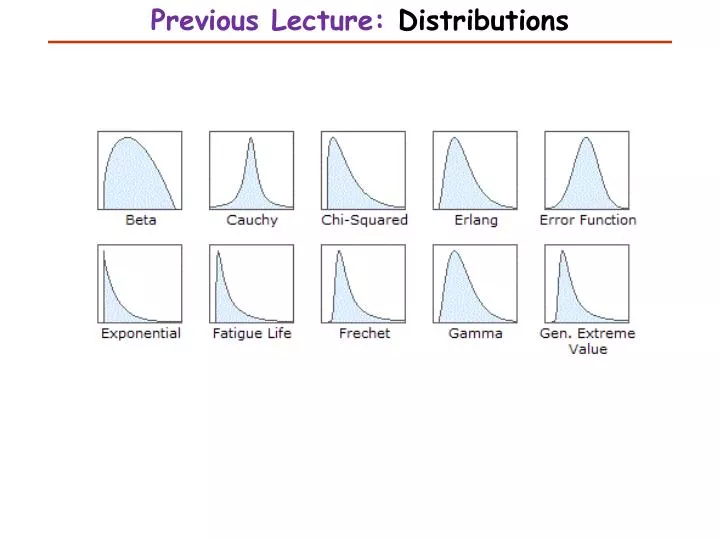
Previous Lecture: Distributions. This Lecture. Introduction to Biostatistics and Bioinformatics Estimation I. By Judy Zhong Assistant Professor Division of Biostatistics Department of Population Health Judy.zhong@nyumc.org.

E N D
This Lecture Introduction to Biostatistics and Bioinformatics Estimation I By Judy Zhong Assistant Professor Division of Biostatistics Department of Population Health Judy.zhong@nyumc.org
Statistical inference can be further subdivided into the two main areas of estimation and hypothesis Estimation is concerned with estimating the values of specific population parameters Hypothesis testing is concerned with testing whether the value of a population parameter is equal to some specific value Statistical inference
Suppose we measure the systolic blood pressure (SBP) of a group of patients and we believe the underlying distribution is normal. How can the parameters of this distribution (µ, ^2) be estimated? How precise are our estimates? Suppose we look at people living within a low-income census tract in an urban area and we wish to estimate the prevalence of HIV in the community. We assume that the number of cases among n people sampled is binomially distributed, with some parameter p. How is the parameter p estimated? How precise is this estimate? Two examples of estimation
Sometimes we are interested in obtaining specific values as estimates of our parameters (along with estimation precise). There values are referred to as point estimates Sometimes we want to specify a range within which the parameter values are likely to fall. If the range is narrow, then we may feel our point estimate is good. These are called interval estimates Point estimation and interval estimation
Purpose of inference: Make decisions about population characteristics when it is impractical to observe the whole population and we only have a sample of data drawn from the population From Sample to Population! Population?
Parameter: a number describing the population Statistic: a number describing a sample Statistical inference: Statistic Parameter Towards statistical inference
Inference Process Population Estimates & tests Sample statistic Sample
We have a sample (x1, x2, …, xn) randomly sampled from a population The population mean µ and variance ^2 are unknown Question: how to use the observed sample (x1, …, xn) to estimate µ and ^2? Section 6.5: Estimation of population mean
A natural estimator for estimating population mean µ is the sample mean A natural estimator for estimating population standard deviation is the sample standard deviation Point estimator of population mean and variance
To understand what properties of make it a desirable estimator for µ, we need to forget about our particular sample for the moment and consider all possible samples of size n that could have been selected from the population The values of in different samples will be different. These values will be denoted by The sampling distribution of is the distribution of values over all possible samples of size n that could have been selected from the study population Sampling distribution of sample mean
We can show that the average of these samples mean ( over all possible samples) is equal to the population mean µ Unbiasedness: Let X1, X2, …, Xn be a random sample drawn from some population with mean µ. Then Sample mean is an unbiased estimator of population mean
The unbiasedness of sample mean is not sufficient reason to use it as an estimator of µ There are many other unbiasedness, like sample median and the average of min and max We can show that (but not here): among all kinds of unbiased estimators, the sample mean has the smallest variance Now what is the variance of sample mean ? is minimum variance unbiased estimator of µ
The variance of sample mean measures the estimation precise Theorem: Let X1, …, Xn be a random sample from a population with mean µ and variance . The set of sample means in repeated random samples of size n from this population has variance . The standard deviation of this set of sample means is thus and is referred to as the standard error of the mean or the standard error. Standard error of mean
In practice, the population variance is rarely unknown. We will see in Section 6.7 that the sample variance is a reasonable estimator for Therefore, the standard error of mean can be estimated by (recall that ) NOTE: The larger sample size is the smaller standard error is the more accurate estimation is Use to estimate
A sample of size 10 birthweights: 97, 125, 62, 120, 132, 135, 118, 137, 126, 118 (sample mean x-bar=117.00 and sample standard deviation s=22.44) In order to estimate the population mean µ, a point estimate is the sample mean , with standard error given by An example of standard error
Let X1, …, Xn be a random sample from a population with µ and σ2 . Then the mean and variance of is µ and σ2/n, respectively Furthermore, if X1, ..., Xn be a random sample from a normal population with µ and σ2 . Then by the properties of linear combination, is also normally distributed, that is Now the question is, if the population is NOT normal, what is the distribution of ? Summary of sampling distribution of
Let X1 , X2 , …, Xn denote n independent random variables sampled from some population with mean and variance 2 When n is large, the sampling distribution of the sample mean is approximately normally distributed even if the underlying population is not normal By standardization: The Central Limit Theorem
Example 6.27 (Obstetrics example continued) Compute the An example of using CLT
Let X1 , X2 , …, Xn denote n independent random variables sampled from some population with mean and variance 2 Our goal is to estimate µ. We know that is a good point estimate Now we want to have a confidence interval such that Interval estimation
From Central Limit Theorem, we have But we still cannot use this to construct interval estimation for µ, because is unknown Now we replace by sample standard deviation s, what is the distribution of the following? Motivation for t-distribution
If X1, …, Xn ~ N(µ,2) and are independent, then where is called t-distribution with n-1 degrees of freedom T-distribution
See Table 5 in Appendix The (100×u)th percentile of a t distribution with d degrees of freedom is denoted by That is T-table
The bigger degrees of freedom, the closer to the standard normal distribution Comparison of normal and t distributions
100%×(1-α) area 1-α α/2 α/2 tα/2 =-t1-α/2 t1-α/2 • Define the critical values t1-α/2 and -t1-α/2 as follows
We start from Our goal is get a 95% interval estimation
Confidence Interval for the mean of a normal distribution A 100%×(1-α) CI for the mean µ of a normal distribution with unknown variance is given by A shorthand notation for the CI is Confidence interval
Confidence Interval for the mean of a normal distribution (large sample case) A 100%×(1-α) CI for the mean µ of a normal distribution with unknown variance is given by A shorthand notation for the CI is Confidence interval (when n is large)