Download
1 / 35
350 likes | 501 Vues
A receding horizon genetic algorithm for dynamic multi-target assignment and tracking. A case study on the optimal positioning of tug vessels along the northern Norwegian coast. Robin T. Bye, Assoc. Prof. Dept. of Technology and Nautical Sciences Ålesund University College (ÅUC) Norway.

E N D
A receding horizon genetic algorithm for dynamic multi-target assignment and tracking A case study on the optimal positioning of tug vessels along the northern Norwegian coast Robin T. Bye, Assoc. Prof. Dept. of Technology and Nautical Sciences Ålesund University College (ÅUC) Norway
Introduction • Multiple agents are to be (a) assigned and (b) track multiple moving targets in a dynamic environment • (a) Target assignment/resource allocation: • which agents shall track which targets? • (b) Collective tracking/positioning: • how should the agents move to increase net tracking performance or minimise cost? Robin T. Bye, Ålesund University College
Introduction cont’d • Tracking performance: • how to define a cost measure? • Dynamic environment: • how can agents respond to • targets changing their trajectories? • new targets appearing and/or targets disappearing? • variable external conditions? Robin T. Bye, Ålesund University College
Case study: Positioning of tugs • Norwegian Coastal Administration (NCA) • runs a Vessel Traffic Services (VTS) centre in Vardø • monitors ship traffic off northern Norwegian coast with the automatic identification system (AIS) • commands a fleet of patrolling tug vessels • Patrolling tug vessels (=agents) • must stop drifting oil tankers (=targets) or other ships and tow them to safety before grounding • are instructed by NCA to go to “good” positions that (hopefully) reduce the risk of drift grounding accidents Robin T. Bye, Ålesund University College
Automatic identification system (AIS) • Ships required to use AIS by law • Real-time VHF radio transmission to VTS centres • Static info: ID, destination, cargo, size, etc. • Dynamic info: Speed, position, heading, etc. • Enables prediction of future state of ships (e.g., position, speed, rate of turn) Robin T. Bye, Ålesund University College
Dynamical risk models of NCA • Risk-based decision support tools • Based on static information • type of ships, cargo, crew, nationality, etc. • geography, e.g., known dangerous waters • … and dynamic information • Ships’ position, direction, speed, etc. • weather conditions, e.g., wind, currents, waves, etc. Robin T. Bye, Ålesund University College
Dynamical risk models of NCA Courtesy NCA Robin T. Bye, Ålesund University College
Dynamical risk models of NCA Courtesy NCA Robin T. Bye, Ålesund University College
Motivation • Today: Human operator makes decisions based on dynamical risk models • Limitation: Requires small number of tankers and tugs to be manageable by human operator • Oil/gas development in northern waters will increase traffic in years to come How should a fleet of tugs move to reduce risk of accidents? • Algorithm needed for optimising tug positioning Robin T. Bye, Ålesund University College
Oil tanker traffic • Traffic: Along corridors • Tugs: Near shore • We can approximate corridors by parallel lines Courtesy NCA Robin T. Bye, Ålesund University College
Problem description • Lines of motion for 3 oil tankers (white) and 2 patrol tugs (black) • Predicted drift paths at future points in time • How should tugs move? Robin T. Bye, Ålesund University College
Example scenario Robin T. Bye, Ålesund University College
Scenario explanation • Crosspoint: Where drift trajectory of a tanker crosses patrol line of tugs • Typical drift time: 8-12 hours before crossing of patrol line entering high-risk zone • White circles: Predicted crosspoints of drift trajectories of 6 oil tankers • Prediction horizon Th=24 hours ahead • Black circles: Suboptimal trajectories of 3 tugs How to optimise tug trajectories? Robin T. Bye, Ålesund University College
Method • Examine a finite number of potential patrol trajectories and evaluate a cost function for each • Use a genetic algorithm to find good solutions in reasonable time • Use receding horizon control to incorporate a dynamic environment and update trajectories • Plan trajectories 24 hours ahead but only execute first hour, then replan and repeat Robin T. Bye, Ålesund University College
Genetic algorithm (GA) • Employs the usual GA scheme: • Define cost function, chromosome encoding and set GA parameters, e.g., mutation, selection • Generate an initial population of chromosomes • Evaluate a cost for each chromosome • Select mates based on a selection parameter • Perform mating • Perform mutation based on a mutation parameter • Repeat from Step 3 until desired cost level reached Robin T. Bye, Ålesund University College
Some GA features • Population size: Number of chromosomes • Selection: Fraction of chromosomes to keep for survival and reproduction • Mating: Combination of extrapolation and crossover, single crossover point • Mutation rate: Fraction of genes mutated at every iteration Robin T. Bye, Ålesund University College
Cost function • Sum of distances between all crosspoints and nearest patrol points (positions of tugs) • only care about nearest tug that can save tanker • Define ytp as pth tug’s patrol point at time t • Define ytc as cth tanker’s cross point at time t • Consider No oil tankers and Np patrol tugs Function of time t and chromosome Ci: Robin T. Bye, Ålesund University College
Cost function cont’d cross point cost nearest patrol point Robin T. Bye, Ålesund University College
Chromosome encoding • Contains possible set of Np control trajectories: • Each control trajectory u1p,…,uThpis a sequence of control inputs with values between -1 (max speed south) and +1 (max speed north) • Sequence of patrol points for tug p at time t from difference equation (ts is sample time): Robin T. Bye, Ålesund University College
Receding horizon genetic algorithm (RGHA) • Scenario changes over time: • Winds, ocean currents, wave heights, etc. • Tanker positions, speeds, directions, etc. • Must reevaluate solution found by GA regularly receding horizon control: • Calculate (sub)optimal set of trajectories with duration Th (24 hours, say) into the future • Execute only first part (1 hour, say) of trajectories • Repeat from Step 1 given new and predicted information Robin T. Bye, Ålesund University College
Simulationstudy Robin T. Bye, Ålesund University College
Simulation example, td=0 hours Robin T. Bye, Ålesund University College
Simulation example, td=10 hours Robin T. Bye, Ålesund University College
Simulation example, td=25 hours Robin T. Bye, Ålesund University College
Results • Mean cost • Static strategy: 2361 • RHGA: 808 • Performance improvement: 65.8% • Standard deviation • Static strategy: 985 • RHGA: 292 • Improvement: 70.4% Robin T. Bye, Ålesund University College
Conclusions • The RHGA is able to simultaneously perform multi-target allocation and tracking in a dynamic environment • The choice of cost function gives good tracking with target allocation “for free” (need no logic) • The RHGA provides good prevention against possible drift accidents by accounting for the predicted future environment Robin T. Bye, Ålesund University College
Future directions • Comparison with other algorithms • Extend/change cost function • punish movement/velocity changes (save fuel) • vary risk factor (weight) of tankers • use a set of various max speeds for tankers/tugs • Incorporate boundary conditions • Add noise and nonlinearities • Extend to 2D and 3D • Test with other/faster systems Robin T. Bye, Ålesund University College
Questions? ÅUC campus Robin T. Bye, roby@hials.no Virtual Møre project, www.virtualmore.org Ålesund University College, www.hials.no Robin T. Bye, Ålesund University College
Results Robin T. Bye, Ålesund University College
Simulation example, td=0 hours Robin T. Bye, Ålesund University College
Simulation example, td=5 hours Robin T. Bye, Ålesund University College
Simulation example, td=10 hours Robin T. Bye, Ålesund University College
Simulation example, td=15 hours Robin T. Bye, Ålesund University College
Simulation example, td=20 hours Robin T. Bye, Ålesund University College
Simulation example, td=25 hours Robin T. Bye, Ålesund University College