Orthogonal Functions and Fourier Series

1. CHAPTER 12 Orthogonal Functions and Fourier Series

2. Contents • 12.1 Orthogonal Functions • 12.2 Fourier Series • 12.3 Fourier Cosine and Sine Series • 12.4 Complex Fourier Series • 12.5 Strum-Liouville Problems • 12.6 Bessel and Legendre Series

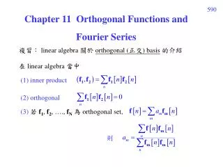
3. DEFINITION 12.2 Orthogonal Function Two functions f1 and f2 are said to be orthogonal on an interval [a, b] if 12.1 Orthogonal Functions DEFINITION 12.1 Inner Product of Function The inner product of two functions f1 and f2on an interval [a, b] is the number

4. Example • The function f1(x) = x2, f2(x) = x3 are orthogonal on the interval [−1, 1] since

5. DEFINITION 12.3 Inner Product of Function A set of real-valued functions {0(x), 1(x), 2(x), …} is said to be orthogonalon an interval [a, b] if (2)

6. Orthonormal Sets • The expression (u, u) = ||u||2 is called the square norm. Thus we can define the square norm of a function as (3)If {n(x)} is an orthogonal set on [a, b] with the property that ||n(x)|| = 1 for all n, then it is called an orthonormal set on [a, b].

7. Example 1 Show that the set {1, cos x, cos 2x, …} is orthogonal on [−, ]. SolutionLet 0(x) = 1, n(x) = cos nx, we show that

8. Example 1 (2) and

9. Example 2 Find the norms of each functions in Example 1. Solution

10. Vector Analogy • Recalling from the vectors in 3-space that (4)we have (5)Thus we can make an analogy between vectors and functions.

11. Orthogonal Series Expansion • Suppose {n(x)} is an orthogonal set on [a, b]. If f(x) is defined on [a, b], we first write as (6)Then

12. Since {n(x)} is an orthogonal set on [a, b], each term on the right-hand side is zero except m = n. In this casewe have

13. In other words, (7) (8)Then (7) becomes (9)

14. DEFINITION 12.4 • Under the condition of the above definition, we have (10) (11) A set of real-valued functions {0(x), 1(x), 2(x), …} is said to be orthogonal with respect to a weight function w(x) on [a, b], if Orthogonal Set/Weight Function

15. Complete Sets • An orthogonal set is complete if the only continuous function orthogonal to each member of the set is the zero function.

16. 12.2 Fourier Series • Trigonometric SeriesWe can show that the set (1)is orthogonal on [−p, p]. Thus a function f defined on [−p, p] can be written as (2)

17. Now we calculate the coefficients. (3)Since cos(nx/p) and sin(nx/p) are orthogonal to 1 on this interval, then (3) becomes Thus we have (4)

18. In addition, (5)by orthogonality we have

19. andThus (5) reduces to and so (6)

20. Finally, if we multiply (2) by sin(mx/p) and useand we find that (7)

21. DEFINITION 12.5 Fourier Series The Fourier series of a function f defined on the interval (−p, p) is given by (8)where (9) (10) (11)

22. Example 1 Expand (12)in a Fourier series. SolutionThe graph of f is shown in Fig 12.1 with p = .

23. Example 1 (2) ←cos n = (-1)n

24. Example 1 (3) From (11) we haveTherefore (13)

25. Fig 12.1

26. THEOREM 12.1 Let f and f’ be piecewise continuous on the interval (−p, p); that is, let f and f’ be continuous except at a finite number of points in the interval and have only finite discontinuous at these points. Then the Fourier series of f on the interval converge to f(x) at a point of continuity. At a point of discontinuity, the Fourier series converges to the averagewhere f(x+) and f(x－) denote the limit of f at x from the right and from the left, respectively. Criterion for Convergence

27. Example 2 • Referring to Example 1, function f iscontinuous on (−, ) except at x = 0. Thus the series (13) will converge to at x = 0.

28. Periodic Extension • Fig 12.2 is the periodic extension of the function f in Example 1. Thus the discontinuity at x = 0, 2, 4, …will converge toand at x = , 3, … will converge to

29. Fig 12.2

30. Sequence of Partial Sums • Sequence of Partial SumsReferring to (13), we write the partial sums asSee Fig 12.3.

31. Fig 12.3

32. 12.3 Fourier Cosine and Sine Series • Even and Odd Functions • even if f(−x) = f(x) • odd if f(−x) = −f(x)

33. Fig 12.4 Even function

34. Fig 12.5 Odd function

35. THEOREM 12.2 (a) The product of two even functions is even. (b) The product of two odd functions is even. (c) The product of an even function and an odd function is odd. (d) The sum (difference) of two even functions is even. (e) The sum (difference) of two odd functions is odd. (f) If f is even then (g) If f is odd then Properties of Even/Odd Functions

36. Cosine and Sine Series • If f is even on (−p, p) thenSimilarly, if f is odd on (−p, p) then

37. DEFINITION 12.6 (i) The Fourier series of an even function f on the interval (−p, p) is the cosine series (1)where (2) (3) Fourier Cosine and Sine Series

38. (continued) DEFINITION 12.6 (ii) The Fourier series of an odd function f on the interval (−p, p) is the sine series (4)where (5) Fourier Cosine and Sine Series

39. Example 1 Expand f(x) = x, −2 < x < 2 in a Fourier series. SolutionInspection of Fig 12.6, we find it is an odd function on (−2, 2) and p = 2. Thus (6)Fig 12.7 is the periodic extension of the function in Example 1.

40. Fig 12.6

41. Fig 12.7

42. Example 2 • The functionshown in Fig 12.8 is odd on (−, ) with p = .From (5), and so (7)

43. Fig 12.8

44. Gibbs Phenomenon • Fig 12.9 shows the partial sums of (7). We can see there are pronounced spikes near the discontinuities. This overshooting of SN does not smooth out but remains fairly constant even when N is large. This is so-called Gibbs phenomenon.

45. Fig 12.9

46. Half-Range Expansions • If a function f is defined only on 0 < x < L, we can make arbitrary definition of the function on −L < x < 0. • If y = f(x) is defined on 0 < x < L, • reflect the graph about the y-axis onto −L < x < 0; the function is now even. See Fig 12.10. • reflect the graph through the origin onto −L < x < 0; the function is now odd. See Fig 12.11. • define f on −L < x < 0 by f(x) = f(x + L). See Fig 12.12.

47. Fig 12.10

48. Fig 12.11

49. Fig 12.12

50. Example 3 Expand f(x) = x2, 0 < x < L, (a) in a cosine series, (b) in a sine series (c) in a Fourier series. SolutionThe graph is shown in Fig 12.13.