Download
1 / 54
540 likes | 1.04k Vues
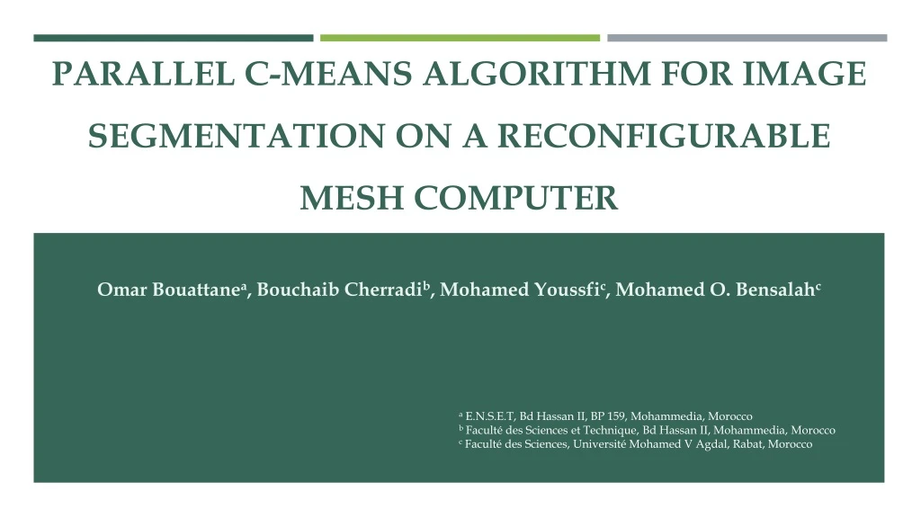
Parallel c-means algorithm for image segmentation on a reconfigurable mesh computer. Omar Bouattane a , Bouchaib Cherradi b , Mohamed Youssfi c , Mohamed O. Bensalah c. a E.N.S.E.T, Bd Hassan II, BP 159, Mohammedia , Morocco

E N D
Parallel c-means algorithm for image segmentation on a reconfigurable mesh computer Omar Bouattanea, BouchaibCherradib, Mohamed Youssfic, Mohamed O. Bensalahc a E.N.S.E.T, Bd Hassan II, BP 159, Mohammedia, Morocco b Faculté des Sciences et Technique, Bd Hassan II, Mohammedia, Morocco c Faculté des Sciences, Université Mohamed V Agdal, Rabat, Morocco
Abstract. The authors propose a parallel algorithm for data classification, and its application for Magnetic Resonance Images (MRI) segmentation. The studied classification method is the well-known c-means method. The use of the parallel architecture in the classification domain is introduced in order to improve the complexities of the corresponding algorithms, so that they will be considered as a pre-processing procedure. The proposed algorithm is assigned to be implemented on a parallel machine, which is the reconfigurable mesh computer (RMC). The image of size (mn) to be processed must be stored on the RMC of the same size, one pixel per processing element (PE).
1. Introduction. Image segmentation is a splitting process of images into a set of regions, classes or homogeneous sub-sets according to some criteria. Usually, gray levels, texture or shapes constitute the well-used segmenting criteria. Their choice is frequently based on the kind of images and the goals to be reached after processing. Image segmentation can be considered as an image processing problem or a pattern recognition one. In the case of image processing consideration, we distinguish two essential approaches that are: region approach and contour approach. In the first approach, we look for homogeneous regions using some basic techniques such as thresholding, region growing, morphological mathematics and others [1]. [1] H.D. Heng, X.H. Jiang, Y. Sun, J. Wang, Color image segmentation: advances and prosoects, Pattern Recognition 34 (2001) 2259–2281.
I. Introduction – cont. Thresholding technique discriminates pixels using their gray levels. It supposes implicitly that intensity structures are sufficiently discriminative, and guarantee good separation [2]. [2] A. Zijdenbos, B. M. Dawant, Brain segmentation and white matter lesion detection in MR images, Critical Reviews in Biomedical Engineering 22 (5/6) (1994) 401–465. In [3] the authors propose a multi-modal histogram thresholding method for gray-level images. [3] J. H. Chang, K. C. Fan, Y. L. Chang, Multi-modal gray-level histogram modeling and decomposition, Image and Vision Computing 20 (2002) 203–216. Region growing technique is based on progressive aggregations of pixels starting from a given point named ‘‘germ’’. In [4] the authors propose a region growing method for cervical 3-D MRI image segmentation. [4] J.P. Thiran et al., A queue-basedregiongrowingalgorithm for accuratesegmentation of multi-dimensional digital images, Signal Processing 60 (1997)1–10. The proposed algorithm combines the automatic selection of germs with a growing regions procedure that is based on the ‘‘watershed’’ principle.
I. Introduction – cont. Morphological mathematics techniques based on erosion, dilation, closure and opening operations are also used in segmentation problems. It was used in [5] to isolate the cerebral overlap for MRI images. [5] J.-F.Mangin, Robust brainsegmentationusinghistogram scale-spaceanalysisandmathematicalmorphology, in: MICCAI’98 First International Conference on Medical ImageComputingand Computer AssistedIntervention, 1998, pp. 1230–1241. In [6] the authors propose an MR image segmentation algorithm for classifying brain tissues. [6] C. Tsai, B.S. Manjunath, R. Jagadeesan, Automated segmentation of brain MR images, Pattern Recognition 28 (12) (1995) 1825–1837. Their method associates the adaptive histogram analysis, morphological operations and knowledge based rules to sort out various regions such as the brain matter and the cerebrospinal fluid, and detect if there are any abnormal regions.
I. Introduction – cont. In the contour approach case, some derivative operators are used at first to sort out discontinuities on image, on the other hand, some deformable models coming from dynamic contours methods are introduced in [7, 8]. [7] D. Terzopoulos et al, Snakes: active contour models, International Journal of Computer Vision (1988) 321–331. [8] D. Terzopoulos et al, Deformablemodels in medical imageanalysis: a survey, Medical ImageAnalysis 1 (2) (1996) 91–108. The latter have some advantages comparing to the first by the fact that, they deliver the closed contours and surfaces. In the case of the pattern recognition point of view, the problem is to classify a set of elements defined by a set of features among which a set of classes can be previously known. In the MRI segmentation domain, the vector pattern X corresponds to the gray level of the studied point (pixel). From these approaches, one distinguishes the supervised methods where the class features are known a priori, and the unsupervised ones which use the features auto-learning.
I. Introduction – cont. From this point of view, several algorithms have been proposed such as: c-means, fuzzy c-means (FCM) [9], adaptive c-means [10], modified fuzzy c-means [11] using illumination patterns and fuzzy c-means combined with neutrosophic set [12]. [9] J.S.R. Jang, C. Sun, T.E. Mizutani, Neuro-Fuzzy and Soft Computing, PrenticeHall, 1997. pp. 426–427. [10] L. Dzung Pham, L.P. Jerry, An adaptative fuzzy c means algorithm for image segmentation in the presence of intensity inhomogeneities, Pattern RecognitionLetters 20 (1999) 57–68. [11] L. Ma, R.C. Staunton, A modified fuzzy c-meansimagesegmentationalgorithm for usewithunevenilluminationpatterns, Pattern Recognition 40(2007) 3005–3011. [12] Y. Guo, H.D. Cheng, W. Zaho, Y. Zhang, A novelimagesegmentationalgorithmbased on fuzzy c-meansalgorithmandneutrosophic set, in: Proceeding of the 11th Joint Conference on Information Sciences, Atlantis Press, 2008. Segmentation is a very large problem; it requires several algorithmic techniques and different computational models, which can be sequential or parallel using processor elements, cellular automata or neural networks. Improvement and parallelism of c-means clustering algorithm was presented in [19] to demonstrate the effectiveness and how the complexity of the parallel algorithm can be reduced in the Single Instruction Multiple Data (SIMD) computational model. [19] J. Tian et al, Improvement and parallelism of k-means clustering algorithm, Tsinghua Science and Technology 10 (3) (2005) 277–281. ISSN 1007-0214, 01/21.
I. Introduction – cont. In the literature, there are several parallel approaches to implement the clustering algorithms. The difference from one to another method is how to exploit the parallelism feasibilities and the huge programming field offered by various parallel architectures to achieve effective solutions and subsequently the reduced complexity algorithms. Notice that all the steps of the well known c-means clustering algorithm are generally identical but they are implemented differently by authors according to the parallel architecture used as a computational model. For example, in [20] authors have proposed a parallel approach using a hardware VLSI systolic architecture. [20] L.M. Ni, A.K. Jain, A VLSI systolic architecture for pattern clustering, IEEE Transaction on Pattern Analysis and Machine Intelligence (1985) 79–89. In their proposed method, the c-means clustering problem is subdivided into several elementary operations that are organized in a pipeline structure, and the resulted schemes of the obtained logic cells are also associated to design the processing modules of a hardware circuit for clustering problem. This solution was argued by a simulation experiments to evaluate the effectiveness of the proposed systolic architecture.
I. Introduction – cont. Another strategy was proposed in [21] where the authors have started by presenting a set of basic data manipulation operations using reconfiguration properties of the reconfigurable mesh (RMESH). [21] J.F. Jenq, S. Sahni, Reconfigurable mesh algorithms for image shrinking, expanding, clustering and template matching, International Parallel Processing Symposium (1991) 208–215. These basic operations are also used to elaborate some parallel data processing procedures in order to implement the parallel clustering algorithm. The problem of data clustering was studied and detailed for a general case of N vector patterns. The proposed complexity for their method is O(Mk + klogN) where k is the number of clusters, M is the size of the vector features of each data point and N is the size of the input data set which is the same as the RMESH size.
I. Introduction – cont. Another strategy was proposed in [21] where the authors have started by presenting a set of basic data manipulation operations using reconfiguration properties of the reconfigurable mesh (RMESH). [21] J.F. Jenq, S. Sahni, Reconfigurable mesh algorithms for image shrinking, expanding, clustering and template matching, International Parallel Processing Symposium (1991) 208–215. These basic operations are also used to elaborate some parallel data processing procedures in order to implement the parallel clustering algorithm. The problem of data clustering was studied and detailed for a general case of N vector patterns. The proposed complexity for their method is O(Mk + klogN) where k is the number of clusters, M is the size of the vector features of each data point and N is the size of the input data set which is the same as the RMESH size.
I. Introduction – cont. In [22] the authors have proposed an optimal solution for parallel clustering on a reconfigurable array of processors. [22] H.R. Tsai, S.J. Horng, Optimal parallel clustering algorithms on a reconfigurable array of processors with wider bus networks, Image and Vision Computing (1999) 925–936. The proposed approach is based on the same strategy that divides the clustering problem into a set of elementary operations. Each of these elementary operations is implemented on wider communication bus architecture to reach an optimal run time complexity. Also, some basic operations are translated into shifting operation in the same wider bus network to achieve O(1) time complexity in order to optimize the global clustering algorithm complexity.
I. Introduction – cont. In the same way, using the same strategy and the same computational model as in [21], the authors propose in this presentation an times parallel algorithm for c-means clustering problem and its application to the MRI cerebral images. [21] J.F. Jenq, S. Sahni, Reconfigurable mesh algorithms for image shrinking, expanding, clustering and template matching, International Parallel Processing Symposium (1991) 208–215. The presented algorithm is assigned to be implemented on a massively parallel reconfigurable mesh computer of the same size as the input image. The corresponding parallel program of the proposed algorithm is validated on a 2-D reconfigurable mesh emulator [23]. [23] M. Youssfi, O. Bouattane, M.O. Bensalah, A massively parallel re-configurable mesh computer emulator: design, modeling and realization, Journal of Software Engineering and Applications 3 (2010) 11–26. Some interesting obtained results and the complexity analysis and an effectiveness features study of the proposed method are also presented.
2. Parallel Computational Model. 2.1. Presentation A reconfigurable mesh computer (RMC) of size n n, is a massively parallel machine having n2 processing elements (PEs) arranged on a 2-D matrix as shown in Figure 1. It is a Single Instruction Multiple Data (SIMD) structure, in which each PE(i,j) is localized in row i and column j and has an identifier defined by ID = ni + j. Each PE of the mesh is connected to its four neighbors (if they exist) by communication channels. It has a finite number of registers of size (log2n) bits. The PEs can carry out arithmetic and logical operations. They can also carry out reconfiguration operations to exchange data over the mesh.
2. Parallel Computational Model - cont. 2.2. Basic operations of a PE 2.2.1. Arithmeticoperations Like any processor, each processing element (PE) of the RMC possesses an instruction set relating to the arithmetic and logical operations. The operands concerned can be the local data of a PE or the data arising on its communication channels after any data exchange operation between the PEs. 2.2.2. Configurationoperations In order to facilitate data exchange between the PE’s over the RMC, each PE possesses an instruction set relating to the reconfiguration and switching operations. Below, we enumerate all the possible reconfiguration operations that can carry out any PE of the RMC according to its usefulness in any stage of any algorithm.
2. Parallel Computational Model - cont. Figure 1: A reconfigurable mesh computer of size 8 8.
2. Parallel Computational Model - cont. • Simple bridge (SB): • A PE of the RMC is in a given state of SB if it establishes connections between two of its communication channels. This PE can connect itself to each bit of its channels, either in transmitting mode, or in receiving mode, as it can be isolated from some of its bits (i.e. neither transmitter, nor receiver). • Various SB configurations of Fig. 2a are described by the following formats:{EW, S, N}, {E, W, SN}, {ES, W, N},{NW, S, E}, {E N, S, W} and {WS, E, N}. E, W, N and S indicate the East, West, North and South Ports of a PE, respectively. • Double bridge (DB): • A PE is in a DB state when it carries out a configuration having two independent buses. • In the same way as in the simple bridge configuration, each PE can connect itself to each bit of its channels, either in transmitting mode, or in receiving mode. Also, it can be isolated from some of its bits (i.e. neither transmitter, nor receiver). • The various possible DB configurations of Fig. 2b are:{EW, NS}, {ES, NW} and {EN, SW}.
2. Parallel Computational Model - cont. • Crossed bridge (CB): • A PE is in CB state when it connects all its active communication channels in only one; each bit with its correspondent. • This operation is generally used when we want to transmit information to a set of PEs at the same time. • The full CB of Fig. 2c.2 is defined by the configuration: {NESW}. • But, the other CB configurations defined by the following formats {E, WNS}, {EWN, S}, {ENS, W}, {EWS, N} are considered as the partial CB configurations, because, in each case, one of the four communication channel of the PE is locked.
2. Parallel Computational Model - cont. Figure 2: Different configurations carried out by the PE’s of the RMC. (a) Simple bridge (SB), (b) double bridge (DB) and (c) crossed bridge (CB).
3. Parallel segmentation algorithm. 3.1. Standardc-meansalgorithm
3. Parallel segmentation algorithm - cont. As presented in [9], the c-means classification is achieved using the following algorithm stages: [9] J.S.R. Jang, C. Sun, T.E. Mizutani, Neuro-Fuzzy and Soft Computing, PrenticeHall, 1997. pp. 426–427. Stage 1: Initialize the class centers Ci, (i = 1,. . ., c). This is carried out by selecting randomly c points in the gray level scale [0 … 255].For eachiterationi: Stage 2: Determine the membership matrix using Eq. 3. Stage 3: Compute the objective function J by Eq. 2. Stage 4: Compare the obtained objective function J to the one computed at iteration i - 1 and stop the loop (i.e. go to stage 6) if the absolute value of the difference between the successive objectives functions is lower than an arbitrary definedthreshold (Sth). Stage 5: Calculate the new class centers using Eq. 6, and return back to perform stages 2, 3 and 4. Stage 6: End.
3. Parallel segmentation algorithm - cont. 3.1. Parallelc-meansalgorithm The authors propose a parallel implementation of the c-means algorithm on a reconfigurable mesh. The input data of the algorithm is an m n MRI cerebral image of 256 gray levels, stored in a reconfigurable mesh of the same size one pixel per PE. In the used computational model, each PE must be equipped by a set of internal registers. These registers will be used during the different stages of the algorithm. They are defined as in the following Table 1. Table 1: The different registers required by a PE to perform the parallel c-means algorithm.
3. Parallel segmentation algorithm - cont. 3.2.1. Initializationprocedure This procedure consists on initializing the set of registers of each PE of the mesh. We have: This means that these registers are initialized by the values of the coordinates i, j of the PE and the gray level Ng of its associated pixel.
3. Parallel segmentation algorithm - cont. 3.2.2. Classdeterminationprocedure This procedure consists of six essential stages which are: 1. Data broadcasting. 2. Distancecomputation. 3. Membershipdecision. 4. Objectivefunctioncomputation. 5. Loop stop test. 6. New class center determination. These various stages are included in a loop as follows: <Beginning of iteration (n)>
3. Parallel segmentation algorithm - cont. – Return to the stage 2 of the distance computation <End of iteration (n)> It is clear that, for each of the six stages of the class determination procedure, the reconfigurable mesh allows us to choose the rapid and safe parallel procedures. We will report the global complexity for one pass of the proposed algorithm to make comparison with the previous works on the similar computational model. Also, we will make a rigorous complexity analysis for one pass and sort out other aspects related to the dynamic evolution of the class cardinality during each pass. This evolution is pursued until the convergence of the algorithm. This aspect will be studied by the proposed parallel classification algorithm for MRI images. Indeed, the MRI images represent interesting data sets which require real time algorithms and high performance computational models such as the massively reconfigurable meshcomputers.
4. Complexity analysis. In order to evaluate the complexity of our parallel algorithm, it is useful to report the complexities of all its stages. They are summarized in Table 2. Table 2: The complexities of each stage of the proposed parallel algorithm.
4. Complexity analysis – cont. The resultedcomplexityis: This complexity depends on the unknown cardinalities of the Cm classes. So, it must be studied according to the c variable to look for its maximum in order to compare it with the well known previous works. For a given c, to reach the maximum of 9 it is necessary to solve the following problem: where N is the total number of points of the input image.
4. Complexity analysis – cont. In order to compare our complexity with those of the previous works, we use the comparison Table 3 as stated in [22]. [22] H.R. Tsai, S.J. Horng, Optimal parallel clustering algorithms on a reconfigurable array of processors with wider bus networks, Image and Vision Computing (1999) 925–936. Table 3: Results of the complexities comparison for parallel clustering.
4. Complexity analysis – cont. In this table the authors were studied the clustering problem by taking into account that each data point must have a number of M features. The number M is used in all the steps of their algorithms. Furthermore, some authors proposed some enhanced solutions by extending the sizes of their computational models. In this paper, the input data set of our algorithm is a gray leveled image, where each point has M = 1 feature (its gray level). This algorithm can be extended easily for any (M >1) features. In this case the complexities of the two first stages of the algorithm (data broadcasting and the first step of the distance computation stage) are altered. They are multiplied by M. Hence, the maximum value of our algorithm complexity becomes:
4. Complexity analysis – cont. Notice that, in the results comparison Table 3, the variable k is used instead of c to represent the same thing. It represents the number of clusters. Table 3 shows the different time complexities for the same clustering problem, using different architectures of the computational models. In this table N represents the size of the input data set also it corresponds to size of the parallel architecture used. For a reduced size computational model, N remains the size of the data set and P is the size of parallel architecture used; M is the vector features size of the data point. For a rigorous comparison, we must compare our results with those obtained by authors of [21], because they used the same computational model RMESH of the same size and the same Bus width. Thus, we can easily show that the obtained complexity is less than O(Mk + klogN) obtained in [21]. [21] J.F. Jenq, S. Sahni, Reconfigurable mesh algorithms for image shrinking, expanding, clustering and template matching, International Parallel Processing Symposium (1991) 208–215.
5. Implementation and results. The parallel algorithm, described in Section 3, is implemented in our emulating framework [23] using its parallel programming language. The program code presented in Fig. 3 is performed using the MRI cerebral image as data input. Figure 3: Segmentation results by the elaborated parallel program.
5. Implementation and results - cont. Before its execution, we define in the initialization phase the number of classes by c = 3. This means that the classes looked for in the image are the white matter, the gray matter and the cerebrospinal fluid. The background of the image is not considered by thealgorithm. Parallel c-means program code:
5. Implementation and results - cont. Parallel c-means program code – cont.:
5. Implementation and results - cont. Parallel c-means program code – cont.:
5. Implementation and results - cont. Parallel c-means program code – cont.:
5. Implementation and results - cont. Parallel c-means program code – cont.:
5. Implementation and results - cont. Parallel c-means program code – cont.:
5. Implementation and results - cont. Parallel c-means program code – cont.:
5. Implementation and results - cont. Program results: After performing the presented parallel program, we obtain the following results: the image of Fig. 3a corresponds to a human brain cut, it is the original input image of the program. Figs. 3b–d represent the three matters of the brain. They are named respectively the gray matter, cerebrospinal fluid and white matter. After performing the proposed parallel algorithm, we complete its effectiveness features by the following study which is focused on its dynamic convergence analysis. To do so, we present three cases of study. For each case we use the same input MRI image, but the initial class centers are changed. The results are presented by tables and figures. In the first case, the initial class centers are arbitrarily chosen as: (c1, c2, c3) = (1, 2, 3).
5. Implementation and results - cont. In Table 4, the class centers do not change after 14 iterations and the algorithm converges to the final class centers (c1, c2, c3) = (28.6,101.6,146.03). Notice that, for any iteration, the total number of the image points N is constant. Fig. 4 shows the curves of the different data of Table 4. Theses curves represent the dynamic changes of each class center value and the cardinality of it corresponding class. In Fig. 4a we see clearly the convergence of the class centers. Also, the cardinality of each class is presented in Fig. 4b and the absolute value of the objective function error in Fig. 4c. In the second case, the initial class centers are arbitrarily chosen as: (c1, c2, c3) = (1, 30, 255). In the third case, the initial class centers are arbitrarily chosen as: (c1, c2, c3) = (140,149,150).
5. Implementation and results - cont. Through the obtained results of the three cases of study of Tables 4–6 and represented in Figs. 4–6, we can conclude that the complexity of the presented algorithm is low in term of iteration number, but it depends on the initial class centers. It was discussed in the literature that the c-means algorithm complexity for sequential and parallel strategies can be reduced using some additional preprocessing phases to start from some appropriate class centers. Among the mentioned preprocessing phase, we find the histogramming procedure that orients the class centers towards the histogram modes of the image. The authors do not introduce any preprocessing phase, because the goal is at first, the parallelization of the c-means algorithm and its implementation on a reconfigurable mesh computer emulator to validate the corresponding parallel procedures. In the second time, by the obtained results, we will focus our further studies on the dynamic evolution of the class cardinality from one pass to another until the convergence of the algorithm. Parallel histogram computation algorithms can be easily implemented on the used emulator.
5. Implementation and results - cont. Table 4: Different states of the classification algorithm starting from class centers (c1, c2, c3) = (1, 2, 3).
5. Implementation and results - cont. Figure 4: Dynamic changes of the different classification parameters starting from class centers (c1, c2, c3) = (1, 2, 3). class centers, cardinality of each class, and absolute value of error of the objective function.
5. Implementation and results - cont. Table 5: Different states of the classification algorithm starting from class centers (c1, c2, c3) = (1, 30, 255). Table 6: Different states of the classification algorithm starting from class centers (c1, c2, c3) = (140, 149,150).
5. Implementation and results - cont. Figure 5: Dynamic changes of the different classification parameters starting from the class centers (c1, c2, c3) = (1,30, 255). class centers, cardinality of each class and error of objective function.
5. Implementation and results - cont. Figure 6: Dynamic changes of the different classification parameters starting from class centers (c1, c2, c3) = (140,149,150). class centers, cardinality of each class, and error of objective function.