Download
1 / 12
120 likes | 312 Vues
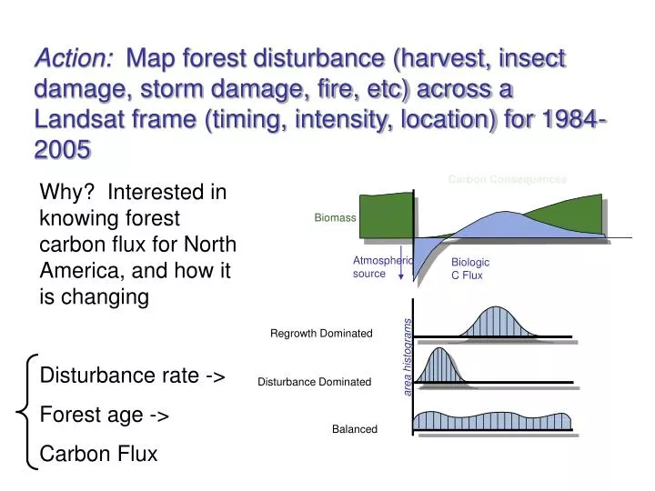
Carbon Consequences. Biomass. Atmospheric source. Biologic C Flux. Regrowth Dominated. area histograms. Disturbance Dominated. Balanced. Action: Map forest disturbance (harvest, insect damage, storm damage, fire, etc) across a Landsat frame (timing, intensity, location) for 1984-2005.

E N D
Carbon Consequences Biomass Atmospheric source Biologic C Flux Regrowth Dominated area histograms Disturbance Dominated Balanced Action: Map forest disturbance (harvest, insect damage, storm damage, fire, etc) across a Landsat frame (timing, intensity, location) for 1984-2005 Why? Interested in knowing forest carbon flux for North America, and how it is changing Disturbance rate -> Forest age -> Carbon Flux
Spatial Sample of US Disturbance Annual or Biennial Image Time Series (1972-2004) Disturbance history / stand age ~25 Sample Sites
Search for leaf-on, cloud-free annual images for a given location; optimize scene selection for anniversary dates. Need to balance: - cloud avoidance - seasonality - data quality (e.g. L7 vs L5) - year selection Download/buy data (Landsat-7 data now free; Landsat-5 by end of year)
III. Orthorectify images to map base using GLS data set and SRTM digital topography; clip images to common X-Y spatial domain - image-image registration essential; orthorectification desirable (facilitates GIS integration with other data) IV. Calibrate each image to radiance, and apply atmospheric correction to convert images to surface reflectance - not essential for change detection, but useful for additional studies (e.g. integration with other sensor data; canopy reflectance modeling)
100 km Atmospheric Correction 1990’s Landsat-5 mosaic TOA reflectance Surface reflectance BOREAS Study Region 100 km 100 km
Find a sample of “mature” forest in each scene either by visual inspection or automated histogram thresholding; obtain mean reflectance and standard deviation for this set of pixels, for each scene • VI. Calculate per-pixel “Forestness Index” for each reflectance image according to: • FI = 1/n * S [(ri – rmf_mean) / rmf_stdev] • Where ri is the reflectance for band i (from 1,n), and rmf_mean, _stdev are the mean and standard deviations of the mature forest band for that image.
(b) Disturbance (a) Permanent forest Forestness index Year index (19xx) (c) Thinning (d) Aforestation (e) Permanent non-forest Time Trajectories of Forestness Index Indicate Forest Dynamics
VII Use rule-based system and thresholds to identify disturbance events (e.g. “if FI increases > 8 and stays >6 for at least three consecutive years, then mark Year 1 as disturbance”). - agriculture identified by frequent large changes in FI value - clouds can be identified as large “single event” changes in FI VIII. Filter maps using sieve filter to remove speckle (single pixel changes).
Fig. 1. (a) Location of samples selected across the conterminous United States, where biennial time series stacks of Landsat images (LTSS) were acquired and analyzed to map forest disturbance over the past three decades. The background forest group map shows that most of the forest groups in the United States have been represented by the samples. (b) An example disturbance map developed using the LTSS in a 28.5-kilometer-square area south of Lake Moultrie in South Carolina. Persisting forest, nonforest, and water are shown in green, gray, and blue, respectively. All other colors represent changes mapped in different years. (c) Percent of forest land disturbed annually, calculated according to the derived disturbance map for the entire South Carolina Landsat scene.