Download
1 / 62
620 likes | 1.04k Vues
Lecture 3: Introduction to Classification. CS 175, Fall 2007 Padhraic Smyth Department of Computer Science University of California, Irvine. Outline. Overview of Classification: examples and applications of classification classification: mapping from features to a class label

E N D
Lecture 3: Introduction to Classification CS 175, Fall 2007 Padhraic Smyth Department of Computer Science University of California, Irvine
Outline • Overview of Classification: • examples and applications of classification • classification: mapping from features to a class label • decision boundaries • training and test data accuracy • the nearest-neighbor classifier • Assignments: • Assignment 2 due Wednesday next week • plotting classification data • k-nearest-neighbor classifiers
Classification • Classification is an important component of intelligent systems • We have a special discrete-valued variable called the class, C • C takes values c, where c = 1, c = 2, …., c = m • for now assume m=2, i.e., 2 classes: c= 1 or c= 2 • Problem is to decide what class an object is • i.e., what value the class variable C is for a given object • given measurements on the object, e.g., A, B, …. • These measurements are called “features” • we wish to learn a mapping from Features -> Class • Notation: • C is the class • A, B, etc (the measurements) are called the “features” (sometimes also called “attributes” or “input variables”)
Classification Functions Feature Values (which are known, measured) Predicted Class Value (true class is unknown to the classifier) a b c Classifier d z We want a mapping or function which takes any combination of values x = (a, b, d, ..... z) and will produce a prediction c, i.e., a function c = f(a, b, d, …. z) which produces a value c=1, c=2,…c=m The problem is that we don’t know this mapping: we have to learn it from data!
Applications of Classification • Medical Diagnosis • classification of cancerous cells • Credit card and Loan approval • Most major banks • Speech recognition • IBM, Dragon Systems, AT&T, Microsoft, etc • Optical Character/Handwriting Recognition • Post Offices, Banks, Gateway, Motorola, Microsoft, Xerox, etc • Email classification • classify email as “junk” or “non-junk” • Many other applications • one of the most successful applications of AI technology
Classification of Galaxies Class 2 Class 1
Feature Vectors and Feature Spaces • Feature Vector: • Say we have 2 features: we can think of the features as a 2-component vector • i.e., a 2-dimensional vector, [a b] • So the features correspond to a 2-dimensional space • (clearly we can generalize to d-dimensional space) • this is called the “feature space” • Each feature vector represents the “coordinates” of a particular object in feature space • If the feature-space is 2-dimensional (for example), and the features a and b are real-valued • we can visually examine and plot the locations of the feature vectors
Data from Multiple Classes • Now consider that we have data from m classes (e.g., m=2) • We can imagine the data from each class being in a “cloud” in feature space • data sets D1 and D2 (sets of points from classes 1 and 2) • data are of dimension d (i.e., d-dimensional vectors) • if d = 2 (2 features), we can plot the data • we should see two “clouds” of data points, one cloud per class
Control Group Anemia Group
Decision Boundaries • What is a Classifier? • A classifier is a mapping from feature space (a d-dimensional vector) to the class labels {1, 2, … m} • Thus, a classifier partitions the feature space into m decision regions • The line or surface separating any 2 classes is the decision boundary • Linear Classifiers • a linear classifier is a mapping which partitions feature space using a linear function (a straight line, or a hyperplane) • it is one of the simplest classifiers we can imagine • in 2 dimensions the decision boundary is a straight line
Class Overlap • Consider two class case • data from D1 and D2 may overlap • features = {age, body temperature}, classes = {flu, not-flu} • features = {income, savings}, classes = {good/bad risk} • common in practice that the classes will naturally overlap • this means that our features are usually not able to perfectly discriminate between the classes • note: with more expensive/more detailed additional features (e.g., a specific test for the flu) we might be able to get perfect separation • if there is overlap => classes are not linearly separable
Classification Accuracy • Say we have N feature vectors • Say we know the true class label for each feature vector • We can measure how accurate a classifier is by how many feature vectors it classifies correctly • Accuracy = percentage of feature vectors correctly classified • training accuracy = accuracy on training data • test accuracy = accuracy on new data not used in training
Training Data and Test Data • Training data • labeled data used to build a classifier • Test data • new data, not used in the training process, to evaluate how well a classifier does on new data • Memorization versus Generalization • better training_accuracy • “memorizing” the training data: • better test_accuracy • “generalizing” to new data • in general, we would like our classifier to perform well on new test data, not just on training data, • i.e., we would like it to generalize well to new data • Test accuracy is more important than training accuracy
Examples of Training and Test Data • Speech Recognition • Training data • words recorded and labeled in a laboratory • Test data • words recorded from new speakers, new locations • Zipcode Recognition • Training data • zipcodes manually selected, scanned, labeled • Test data • actual letters being scanned in a post office • Credit Scoring • Training data • historical database of loan applications with payment history or decision at that time • Test data • you
Some Notation • Training Data • Dtrain = { [x(1), c(1)] , [x(2), c(2)] , …………[x(N), c(N)] } • N pairs of feature vectors and class labels • Feature Vectors and Class Labels: • x(i) is the ith training data feature vector • in MATLAB this could be the ith row of an N x d matrix • c(i) is the class label of the ith feature vector • in general, c(i) can take m different class values, e.g., c = 1, c = 2, ... • Let y be a new feature vector whose class label we do not know, i.e., we wish to classify it.
Nearest Neighbor Classifier • y is a new feature vector whose class label is unknown • Search Dtrain for the closest feature vector to y • let this “closest feature vector” be x(j) • Classify y with the same label as x(j), i.e. • y is assigned label c(j) • How are “closest x” vectors determined? • typically use minimum Euclidean distance • dE(x, y) = sqrt(S (xi - yi)2) • Side note: this produces a “Voronoi tesselation” of the d-space • each point “claims” a cell surrounding it • cell boundaries are polygons • Analogous to “memory-based” reasoning in humans
Geometric Interpretation of Nearest Neighbor 1 2 Feature 2 1 2 2 1 Feature 1
Regions for Nearest Neighbors Each data point defines a “cell” of space that is closest to it. All points within that cell are assigned that class 1 2 Feature 2 1 2 2 1 Feature 1
Nearest Neighbor Decision Boundary Overall decision boundary = union of cell boundaries where class decision is different on each side 1 2 Feature 2 1 2 2 1 Feature 1
How should the new point be classified? 1 2 Feature 2 1 2 ? 2 1 Feature 1
Local Decision Boundaries Boundary? Points that are equidistant between points of class 1 and 2 Note: locally the boundary is (1) linear (because of Euclidean distance) (2) halfway between the 2 class points (3) at right angles to connector 1 2 Feature 2 1 2 ? 2 1 Feature 1
Finding the Decision Boundaries 1 2 Feature 2 1 2 ? 2 1 Feature 1
Finding the Decision Boundaries 1 2 Feature 2 1 2 ? 2 1 Feature 1
Finding the Decision Boundaries 1 2 Feature 2 1 2 ? 2 1 Feature 1
Overall Boundary = Piecewise Linear Decision Region for Class 1 Decision Region for Class 2 1 2 Feature 2 1 2 ? 2 1 Feature 1
Geometric Interpretation of kNN (k=1) ? 1 2 Feature 2 1 2 2 1 Feature 1
More Data Points Feature 2 1 1 1 2 2 1 1 2 2 1 2 1 1 2 2 2 Feature 1
More Complex Decision Boundary 1 In general: Nearest-neighbor classifier produces piecewise linear decision boundaries 1 1 Feature 2 2 2 1 1 2 2 1 2 1 1 2 2 2 Feature 1
K-Nearest Neighbor (kNN) Classifier • Find the k-nearest neighbors to y in Dtrain • i.e., rank the feature vectors according to Euclidean distance • select the k vectors which are have smallest distance to y • Classification • ranking yields k feature vectors and a set of k class labels • pick the class label which is most common in this set (“vote”) • classify y as belonging to this class • Theoretical Considerations • as k increases • we are averaging over more neighbors • the effective decision boundary is more “smooth” • as N increases, the optimal k value tends to increase in proportion to log N
K-Nearest Neighbor (kNN) Classifier • Notes: • In effect, the classifier uses the nearest k feature vectors from Dtrain to “vote” on the class label for y • the single-nearest neighbor classifier is the special case of k=1 • for two-class problems, if we choose k to be odd (i.e., k=1, 3, 5,…) then there will never be any “ties” • “training” is trivial for the kNN classifier, i.e., we just use Dtrain as a “lookup table” when we want to classify a new feature vector • Extensions of the Nearest Neighbor classifier • weighted distances • e.g., if some of the features are more important • e.g., if features are irrelevant • fast search techniques (indexing) to find k-nearest neighbors in d-space
Accuracy on Training Data Training Accuracy = 1/n SDtrain I( o(i), c(i) ) where I( o(i), c(i) ) = 1 if o(i) = c(i), and 0 otherwise Where o(i) = the output of the classifier for training feature x(i) c(i) is the true class for training data vector x(i)
Accuracy on Test Data Let Dtest be a set of new data, unseen in the training process: but assume that Dtest is being generated by the same “mechanism” as generated Dtrain: Test Accuracy = 1/ntestSDtest I( o(j), c(j) ) Test Accuracy is usually what we are really interested in: why? Unfortunately test accuracy is often lower on average than train accuracy Why is this so?
Assignment 2 • Due Wednesday….. • 4 parts • Plot classification data in two-dimensions • Implement a nearest-neighbor classifier • Plot the errors of a k-nearest-neighbor classifier • Test the effect of the value k on the accuracy of the classifier
Data Structure simdata1 = shortname: 'Simulated Data 1' numfeatures: 2 classnames: [2x6 char] numclasses: 2 description: [1x66 char] features: [200x2 double] classlabels: [200x1 double]
Plotting Function function classplot(data, x, y); % function classplot(data, x, y); % % brief description of what the function does % ...... % Your Name, CS 175, date % % Inputs % data: (a structure with the same fields as described above: % your comment header should describe the structure explicitly) % Note that if you are only using certain fields in the structure % in the function below, you need only define these fields in the input comments -------- Your code goes here -------
Nearest Neighbor Classifier function [class_predictions] = knn(traindata,trainlabels,k, testdata) % function [class_predictions] = knn(traindata,trainlabels,k, testdata) % % a brief description of what the function does % ...... % Your Name, CS 175, date % % Inputs % traindata: a N1 x d vector of feature data (the "memory" for kNN) % trainlabels: a N1 x 1 vector of classlabels for traindata % k: an odd positive integer indicating the number of neighbors to use % testdata: a N2 x d vector of feature data for testing the knn classifier % % Outputs % class_predictions: N2 x 1 vector of predicted class values -------- Your code goes here -------