Download
1 / 12
120 likes | 283 Vues
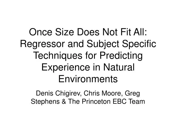
Once Size Does Not Fit All: Regressor and Subject Specific Techniques for Predicting Experience in Natural Environments. Denis Chigirev, Chris Moore, Greg Stephens & The Princeton EBC Team. How do we learn in a very high dimensional setting (~35K voxels) ?. LINEAR. NONLINEAR.

E N D
Once Size Does Not Fit All:Regressor and Subject Specific Techniques for Predicting Experience in Natural Environments Denis Chigirev, Chris Moore, Greg Stephens & The Princeton EBC Team
How do we learn in a very high dimensional setting (~35K voxels) ? LINEAR NONLINEAR Create a “look-up table”: nonlinear kernel methods, kernel ridge regression, RKHS, GP, nonlinear SVM Look for linear projection(s): linear regression, ridge regression, linear SVM How to control for complexity? Need similarity measure between brain states (i.e. kernel) & regularization Assumes “clustering” of similar states Loss function: quadratic linear, hinge Prior (regularization) similarity measure Advantage: pools together many weak signals Assumes regressor continuity along paths of data points weights
How do we learn in a very high dimensional setting (~35K voxels) ? LOCAL GLOBAL Focus on informative areas: choose voxels by correlation thresholding, searchlight Look for global modes: whole brain, PCA, euclidean distance kernel, searchlight kernel without thresholding Advantage: ignore areas that are mostly noise Assumes that information is localized, and feature selection method is stable Advantage: improves stability by pooling over larger areas Disadvantage: correlated noisy areas that do not carry any information may bias the predictor
Different methods emphasize different aspects of the learning problem
Ridge Regression using ALL voxels Difference of means (centroids): Linear regression solution: Ridge regression solution: • Regularization allows to use all ~ 30K voxels • Centroids are well estimated (1st order statistic), but covariance matrix is 2nd order, therefore requires regularization
Whole Brain Ridge Regression Keeping only large eigenvalues of covariance matrix (i.e. PCA-type compexity control) is MUCH LESS effective than ridge regularization.
Reproducing Kernel Hilbert Space (RKHS) T. Poggio Instead of looking for linear projections (ridge regression, SVM w/ linear kernel), use the measure of similarity between brain states to project the new brain state onto existing ones in feature space. where (number of TRs) learn “support” coefficients by solving this equation, where represents regularization in feature space. (aka Kernel Ridge Regression, if use gaussian kernel recover mean GP solution) We choose where is the distance between brain states. We use Euclidean distance and searchlight distance.
How similar are the brain states? Learning algorithm (euclidean distance, mahalanobis, searchlight, earth movers?) (SVM, RKHS, etc. – choice of regularization and loss ) This framework allows the similarity measure between different brain states to be tested for their use in prediction data prediction This allows to assess independently the quality of brain state similarity measure and the quality of the learning procedure. Euclidean measure (default), in practice, performs relatively well.
Basics of Searchlight here is a 3x3x3 “supervoxel”. less different which pair of brain states is further apart? Mahalanobis distance: Problem: amplifies poorly estimated dimension for whole brain states. Solution: apply locally to 3x3x3 supervoxel and then sum individual contributions more different Then the distance between brain states can be computed as a weighted average: We used to find that this solution is now self-regularizing, i.e. one can take the complexity penalty to zero.
Why might searchlight help? (hint: stability!) voxel correlation with feature (movie1 & movie2) Threshold voxel correlation with feature (movie1 & movie2) The projection learned by linear ridge is only as good as the stability of the underlying voxel correlations with the regressor. m2 Searchlight distance versus Euclidean distance, tested in RKHS m1 searchlight correlation with feature (movie1 & movie2) Threshold searchlight corr with feature (movie1 & movie2) m2 m1 m1
Different methods emphasize different aspects of the learning problem
I would like to thank my collaboraters: Chris Moore*, Greg Stephens, Greg Detre, Michael Bannert as well as Ken Norman and Jon Cohen for supporting Princeton EBC Team.