Download

1 / 69
690 likes | 851 Vues
Budget Sampling of Parametric Surface Patches. Jatin Chhugani and Subodh Kumar Johns Hopkins University. Motivation. Sampling a continuous surface into discrete points Rendering as triangles or points FEM/BEM analysis for physics based computation Collision detection

E N D
Budget Sampling of Parametric Surface Patches Jatin Chhugani and Subodh Kumar Johns Hopkins University
Motivation • Sampling a continuous surface into discrete points • Rendering as triangles or points • FEM/BEM analysis for physics based computation • Collision detection • What criteria to satisfy? • Inter-sample distance • Deviation from the actual surface • How to choose the best ‘N’ samples ? • Relationship between the best ‘N’ and the best ‘N+1’ samples?
Example Problem1: Discretise 'AB' into 5 points? Problem 2: Discretise 'AB' into 6 points? A B
Example Common Samples Different Samples Q1 P1 Q2 P2 Q3 P3 Q4 Q5 P4 Q6 P5 Best 6 samples Best 5 samples
Application of Spline Models • CAD/CAM , Entertainment Industry • Medical Visualization • Examples • Submarines • Animation Characters • Human body especially the heart and brain
Interacting with Spline Surfaces • Interactive Spline Rendering: • Need to update image 20-30 times per second • Bound on the number of primitives that can be rendered per second • Interactive Collision Detection: • Need to compute collisions 1000 times per second • Bounded CPU/GPU time • Upper bound on the number of collision tests per second
Interacting with Spline Surfaces • Interactive Spline Rendering: • Need to update image 20-30 times per second • Bound on the number of primitives that can be rendered per second • Interactive Collision Detection: • Need to compute collisions 1000 times per second • Bounded CPU/GPU time • Upper bound on the number of collision tests per second Upper Bound on the number of primitives that can be handled per frame
Issues • Given a threshold (in terms of number of primitives), how to distribute it amongst various parts of the model? • What criteria need to be satisfied? • Plausible image (Minimize artifacts) • Accurate image (or bounded error, quantification if possible) • Bounded Computation Time
Problem Statement Given a set of surface patches {Fi}, and total number of primitives (C), allocate Ci to each patch ensuring fairness. Fairness: Minimize the projected screen-space error of the whole model. Questions: • How to compute Ci to minimize the deviation of samples from surface? • For rendering applications, how to render these primitives?
Rendering Splines • Ray tracing • J. Kajiya ['82], T. Nishita ['90], J. Whitted ['79] • Pixel level surface subdivision • E.Catmull ['74], M. Shantz ['88] • Scan-line based • J. Blinn ['78], J. Lane ['80], J. Whitted ['78] • Polygonal Approximations • Abi-Ezzi ['91], Filip ['86], S. Kumar ['96, '97, '01]
Polygonal Approximations • Produce accurate color and position only at the vertices of the polygons (triangles) • Computationally intensive to figure out tessellation parameters • Maintain expensive data-structures with substantial per-frame update costs • May lead to a large number of small screen-space triangles
Point-Based Rendering • Introduced by Levoy and Whitted ['85] • Explored further by Dally ['98], Rusinkiewicz ['00], Pfister ['00], Stamminger ['01] • Decompose surface into nominally curved `elements` which follow the surface more closely, Szeliski ['92], Witkin ['94], Kalaiah ['01] • Shaded well using algorithms by Zwicker ['01], Kaliah ['02], Adamson ['03]
Point-Based Rendering • No need to maintain topological information • Lower update costs as compared to triangle-based rendering for zoomed-out views • Less beneficial for zoomed-in views
Attributes of each primitive(for Point-Based Rendering) • Position (x,y,z). • Normal (Nx, Ny, Nz). • Color. • Size / Shape ?
Spheres as primitives ImagePlane Spheres on the patch in Object Space Projection of Spheres with no holes Every point on the surface inside at least one sphere.
Rendering Spheres C • Compute the maximum deviation (d) of the projected surface from projection of the center (C). • Draw a square splat of size 2d centered at C.
Our approach 1. Pre-Sampling: • Progressively compute ordered list of samples on the domain of each patch. • Each sample associated with a sphere centered on its corresponding point in 3D. • The radius of the sphere decreases as more points are added.
Our approach 2. View-dependent Point Selection: • Compute the screen-space error for every patch. • Compute the scaling factor for every patch. • Compute the corresponding object-space error. • Search for this value in the sorted list of error values. • Render the corresponding samples with a certain point-size.
Pre-Computation Sampling the Domain Space
Pre-Sampling • Start with the minimal sample set (e.g. the four corners) in the domain. • Generate the 2D Delaunay triangulation.
Pre-Sampling 1 2 3 4 Domain Space
Pre-Sampling • Start with the minimal sample set in the domain. • Generate the 2D Delaunay triangulation. • Compute center and radius of the circumscribing spheres for each triangle (in 3D).
Pre-Sampling 1 2 Point A Point B 3 4 Circumcenter of the triangle
Pre-Sampling • Start with the minimal sample set in the domain. • Generate the 2D Delaunay triangulation. • Compute sphere parameters. • While the sphere with ‘maximum radius’ has radius greater than a user specified parameter: • Append (center, radius) to the list of computed samples. • Update the delaunay triangulation by incrementally adding center and updating the center and radius of the affected triangles.
Pre-Sampling 1 2 Point A Point B 3 4 Circumcenter of the triangle
Pre-Sampling 1 2 5 3 4 Domain Space
Pre-Sampling 1 2 C 5 D B A 3 4 Circumcenter of the triangle
Pre-Sampling 1 2 5 6 3 4 Domain Space
Pre-Sampling Properties • Maximum deviation of a surface patch from the approximating spheres equals the radius of the sphere with the largest radius. • Spheres drawn at the sampled points ensure a hole-free tiling of the surface patch.
What is stored ? • Ordered set of (u,v) pairs • by decreasing deviation • Deviation in object space • i.e., deviation after the sample is added • 3-d Vertex • optional
1. Scaling Factor for a patch Scaling Factor for a vector at point P is the Minimum ratio of the length of the vector to its projected length on the image plane. Q Ratio = Q P P Eye Image Plane
1. Scaling Factor for a patch • Pre-processing • Partition space • For each patch, use the partition containing it • If too many partitions for a patch, subdivide patch • Run-time (for each frame) • Compute the scaling factor for each partition • Scaling factor a patch is that of its partition
2. Budget Allocation per patch Question: Given a screen-space error (α), how to compute the number of points required for a given patch (F)? Solution: • Compute the scaling-factor (). • Compute the object-space error = Δ=(α * ). • Find the index j, such that ΔFj-1 ≥ Δ > ΔFj • Return (j).
Example P1 P2 P3 P4 P5 P6 P7 P8 UV Values Deviation 26 24 21 19 14 13 6 3
Example P1 P2 P3 P4 P5 P6 P7 P8 UV Values Deviation 26 24 21 19 14 13 6 3 Let Δ = 20
Example P1 P2 P3 P4 P5 P6 P7 P8 UV Values Deviation 26 24 21 19 14 13 6 3 Let Δ = 20
Example P1 P2 P3 P4 UV Values Deviation 26 24 21 19 4 samples are chosen such that deviation is less than Δ (20)
2. Budget Allocation per patch Assign a rendering size (d) of 1 initially for every point on each patch. For every frame: • Compute the total points required (C' = Ci). • If C' < C, then done. • Increment d by 1. • Go back to Step 1. Theabove algorithm takes linear time to compute the right rendering size (and hence screen-space error).
2. Budget Allocation per patch (improved) For every frame: 1. Assign the rendering size from the previous frame to every patch 2. Compute the total points required (C' = Ci) 3. If C' < C, then for every patch: a. Decrease its rendering size by 1 b. Recompute C' c. If C' > C return d. Else go back to Step 3
2. Budget Allocation per patch (improved) For every frame: 1. Assign the rendering size from the previous frame to every patch 2. Compute the total points required (C' = Ci) 3. If C' < C, then for every patch: a. Decrease its rendering size by 1 b. Recompute C' c. If C' > C return d. Else go back to Step 3 4. If C' > C, then for every patch: a. Increment its rendering size by 1 b. Recompute C' c. If C' < C return d. Else go back to Step 4
2. Budget Allocation per patch (improved) For every frame: 1. Assign the rendering size from the previous frame to every patch 2. Compute the total points required (C' = Ci) 3. If C' < C, then for every patch: a. Decrease its rendering size by 1 b. Recompute C' c. If C' > C return 4. If C' > C, then for every patch: a. Increment its rendering size by 1 b. Recompute C' c. If C' < C return The above is a 2n-time bounded algorithm exploiting the temporal coherence of the eye points.
3. Rendering Algorithm For every patch: • Project the Ci on the screen using the computed rendering size (d). • In OpenGL: glPointSize(d); glColor3f(…); glNormalPointer(…); glVertexPointer(…); glDrawArrays(GL_POINTS, 0, Ci);
Example Budget: 30 primitives Patch A Patch B Eye Point (E)
Example Rendering Size: 1 pixel 18 Samples 12 Samples Patch A Patch B Eye Point (E)
Example Rendering Size: 1 pixel Holes 18 Samples 12 Samples Patch A Patch B Eye Point (E')
Example Rendering Size: 2 pixels 14 Samples 16 Samples Patch A Patch B Eye Point (E)
Results Pre-comp. Samples Pre-proc. (mts). Patches Model Teapot 32 129,273 09 Goblet 72 123,396 15 Pencil 570 1,051,624 70 Dragon 5,354 1,473,961 96 Garden 38,646 1,231,200 82 Pre-Sampling Performance