Filtering
380 likes | 660 Vues
Filtering. General medical device. gain. sensor. filter. v. gain. Further processing, display, etc. anti-aliasing filter. ADC. Biopotential amplitudes and frequency ranges. Low pass. High pass. 1 st order high pass filter. 1 st order low pass filter. 2 nd order band pass filter.

Filtering
E N D
Presentation Transcript
Filtering 415-4
General medical device gain sensor filter v gain Further processing, display, etc. anti-aliasing filter ADC 415-4
Low pass High pass 415-4
Use filters to pass only signals in the frequency range of interest. • Assume that you are interested in the EMG signal. • A 100 MHz signal from a nearby radio transmitter is interfering with the signal of interest. • Design an RC filter to attenuate the 100 MHz signal. • (Another filter might be need to attenuate low frequency signals.) 415-4
An op amp circuit can filter and amplify at once To analyze: • Convert to phasors. • Use KCL at inverting input. 415-4
An active low pass filter provides more gain at lower frequencies gain Low pass filter 415-4
Measuring magnitude experimentally • |Vo/Vi|=(1+(ωτ)2)-1/2 • Measure output peak-to-peak voltage or RMS voltage (4.1250 V) • Measure input peak-to-peak voltage or RMS voltage (5.9375 V) • f = 3120 Hz 415-4
Measuring phase experimentally • Find period (T=0.32ms) • Find delay between peaks of input and output (-.03ms, -.04 ms) • Convert to degrees, considering there are 360 degrees in one period 415-4
Three different answers! 415-4
Continuous-time low-pass filter • y, Y – output • x, X – input • ωc=1/RC First-order Butterworth 415-4
Discrete-time filtering? filter • Continuous transfer functions can’t describe discrete time signals • Can’t take a derivative of a discrete-time signal x[n] y[n] 415-4
Moving average filter • Say that a signal x[n] is relatively constant except for some random noise which could make it larger or smaller. We can average several samples of x[n] together hoping that the noise would be reduced. • Example: 3 sample moving average filter Output at the current time Input at the current time Input one sample ago Input two samples ago 415-4
FIR filter • Moving average is an example of a finite impulse response (FIR) filter • If the input is an impulse, the output will eventually go to zero • The output depends only on current and past values of the input – we’re filtering in real-time so we can’t use future values. bk are constants and don’t have to equal each other as in the moving average filter M is called the number of “taps” 415-4
FIR filter – 3-point moving average Output (green) is closer to expected value, but is delayed in time from input (blue) Little attenuation in the stop band Linear phase change Better performance with more taps 415-4
Infinite impulse response (IIR) filter • If the input is an impulse, it is possible that the output never reaches zero • The output is a function of both the inputs and past outputs (assuming no gain, which we typically leave out of digital filters) 415-4
IIR filters • Because feedback is used (past outputs contribute to current output) an IIR filter may not be stable • Discrete IIR filters are analogous to circuit filters • RC filter is a first-order Butterworth filter • Other common circuit filter types are Chebyshev and elliptical 415-4
Filter design specs Transition region • In general, all real filters have: • Passband ripple – changes in amplitude in the passband • Transition region – frequency range from passband to stopband • Stopband ripple – changes in amplitude in the stopband • It is typically possible to optimize two of the three Passband ripple magnitude Stopband ripple frequency 415-4
IIR filter types Good transition No ripples in stopband Ripples in passband No ripples Big transition region Sharp transition Ripples in stopband and passband Good transition No ripples in passband Ripples in stopband 415-4
Designing discrete-time filters • Choose what design specs are important for you, then decide what order filter (or number of taps) is feasible with your system • Then, use a tool and let those who know what they are doing do most of the work for you • All of the preceding has assumed lowpass filter, but is applicable with a little tweaking to highpass and bandpass filters From http://zone.ni.com/reference/en-XX/help/371361D-01/lvanlsconcepts/select_dfd/ 415-4
Filters in LabVIEW • Many tools are available that give more or less control over coefficients in the filter equations • Easiest is “Filter Express VI” 415-4
Frequency representation of signals Analog Digital time Time is sampled Frequency is sampled Discrete Fourier Transform (DFT) and inverse DFT allow us to go back and forth • Time is continuous • Frequency is continuous • Fourier transform and inverse Fourier transform allow us to go back and forth 415-4
DFT • DFT operates on N points of a sampled signal • N is chosen long enough to represent all of signal • Result of DFT is a series of complex numbers, X[k] separated by 2π/NT rad/sec (T is sampling period of x[n]) 415-4
Implementing the DFT on a computer • Many calculations are involved in computing the DFT of a discrete-time signal • Fast Fourier Transforms (FFT) are computationally efficient algorithms for finding the DFT • Most FFTs work best when N is a power of 2 • If N is not a power of 2 add zeros (zero padding) to make it so 415-4
Maximum frequency in DFT • The k=N-1 value will be at • ω=2π(N-1)/NT≈2π/T=fs • But recall that when we sample a signal to create x[n] the highest frequency without aliasing is fs/2 • X[0:N/2-1] is mirrored in X[N/2+1:N-1] 415-4
FFT of a rect function Sampling period = 0.2 s N = 16 Frequency resolution = 1.96 rad/s 415-4
How does FFT compare to FT? • We can compare the FFT of a sampled rectfuntion to the FT of a continuous time rect • FT{rect(t/T)} = T sinc(ωT/2) • FFT does an OK approximation – how can we improve it 415-4
Effect of N • N (and sampling frequency) limits the frequency resolution (2π/NT rad/sec) • By choosing only N samples we have “windowed” the signal • Example from continuous time • This widens the frequency spectrum (called spectral leakage) 415-4
“Windowing” and the FFT • Rectangular window • each x[n] (n=0,…,N) is multiplied by 1 • A lot of spectral leakage • Hamming window, Hann window, others • Generally taper to zero at n=0 and n=N • Maximum at n=(N-1)/2 • Reduce spectral leakage • If a default is available, it is generally OK to leave it 415-4
FFT in LabVIEW • Measure the spectrum and display as: • Magnitude peak vs. f • Magnitude RMS vs. f • Power vs. f • Power spectral density (PSD) vs. f • Apply a window (OK to leave as default) • Average many epochs to reduce noise (epoch is a group of N points) 415-4