Download
1 / 29
290 likes | 480 Vues
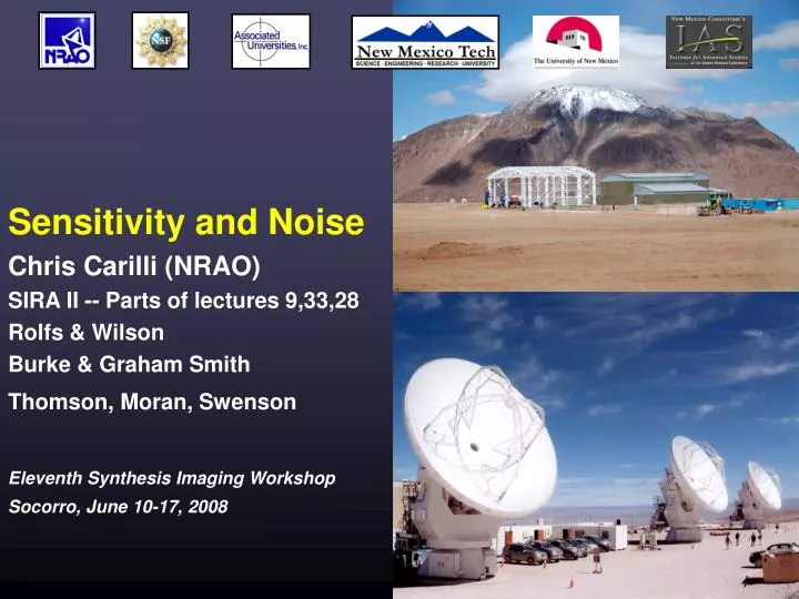
Sensitivity and Noise. Chris Carilli (NRAO) SIRA II -- Parts of lectures 9,33,28 Rolfs & Wilson Burke & Graham Smith Thomson, Moran, Swenson. Some definitions. Interferometric Radiometry Equation. Physically motivate terms Wave noise and photon statistics

E N D
Sensitivity and Noise Chris Carilli (NRAO) SIRA II -- Parts of lectures 9,33,28 Rolfs & Wilson Burke & Graham Smith Thomson, Moran, Swenson
Interferometric Radiometry Equation • Physically motivate terms • Wave noise and photon statistics • Quantum noise (Optical vs. Radio interferometry) • Temperature in Radio Astronomy (Johnson-Nyquist resistor noise, Antenna Temp, Brightness Temp) • Number of independent measurements of TA/Tsys • Some interesting consequences
Photon statistics:Bose-Einstein statistics for gas without number conservation (Reif Chap 9) Thermal equilibrium => Planck distribution function ns = photon occupation number, relative number in state s = number of photons in standing-wave mode in box at temperature T = number of photons/s/Hz in (diffraction limited) beam in free space (Richards 1994, J.Appl.Phys, 76, 1) Photon noise: variance in # photons arriving each second in free space beam
Origin of wave noise: ‘Bunching of Bosons’ in phase space (time and frequency) allows for interference (ie. coherence). h h h Bosons can, and will, occupy the exact same phase space if allowed, such that interference (destructive or constructive) will occur. Restricting phase space (ie. narrowing the bandwidth and sampling time) leads to interference within the beam. This naturally leads to fluctuations that are proportional to intensity (= wave noise).
Origin of wave noise: coherence -- Young’s 2 slit experiment
Origin of wave noise Photon arrival time:normalized probability of detecting a second photoelectron after interval t in a plane wave of linearly polarized light with Gaussian spectral profile of width (Mandel 1963). Exactly the same factor 2 as in Young’s slits! Photon arrival times are correlated on timescales ~ 1/ which naturally leads to fluctuations in the signal total flux, ie. fluctuations are amplified by constructive or destructive interference on timescales ~ 1/
Origin of wave noise III “Think then, of a stream of wave packetseach about c/ long, in a random sequence. There is a certain probability that two such trains accidentally overlap. When this occurs they interfere and one may find four photons, or none, or something in between as a result. It is proper to speak of interference in this situation because the conditions of the experiment are just such as will ensure that these photons are in the same quantum state. To such interference one may ascribe the ‘abnormal’ density fluctuations in any assemblage of bosons. Were we to carry out a similar experiment with a beam of electrons we should find a suppression of the normal fluctuations instead of an enhancement. The accidental overlapping wave trains are precisely the configurations excluded by the Pauli principle.” Purcell 1956, Nature, 178, 1449
When is wave noise important? Photon occupation number at 2.7K Wien RJ
Photon occupation number: examples Bright radio source Optical source Faint radio source
The sky is not dark in the radio! 100 GHz “Even the feeble microwave background ensures that the occupation number at most radio frequencies is already high. In other words, even though the particular contribution to the signal that we seek is very very weak, it is already in a classical sea of noise and if there are benefits to be derived from retaining the associated aspects, we would be foolish to pass them up.” Radhakrishnan 1998
Wave noise: conclusions In radio astronomy, the noise statistics are wave noise dominated, ie. rms fluctuations are proportional to the total power (ns), and not the square root of the power (ns1/2)
Noise limit: quantum noise and coherent amplifiers Phase coherent amplifier automatically puts signal into RJ regime => wave noise dominated Note: phase coherent amplifier is not a detector
Quantum noise of coherent amplifier: nq = 1 Hz-1 s-1 Coherent amplifiers Mirrors + beam splitters Direct detector: CCD ns<<1 => QN disaster, use beam splitters, mirrors, and direct detectors Adv: no receiver noise Disadv: adding antenna lowers SNR per pair as N2 ns>>1 => QN irrelevant, use phase conserving electrons Adv: adding antennas doesn’t affect SNR per pair Disadv: paid QN price
What’s all this about temperatures? Johnson-Nyquist electronic noise of a resistor at TR
Johnson-Nyquist Noise <V> = 0, but <V2> 0 T1 T2 Thermodynamic equil: T1 = T2 • “Statistical fluctuations of electric charge in all conductors produce random variations of the potential between the ends of the conductor…producing mean-square voltage” => white noise power, <V2>/R, radiated from resistor at TR • Transmission line electric field standing wave modes: = c/2l, 2c/2l… Nc/2l… • # modes (=degree freedom) in + : N = 2l / c • Therm. Equipartion law: energy/degree of freedom: E = h/(eh/kT - 1) ~ kT (RJ) • Energy equivalent on line in : E = E N = (kT2l) / c • Transit time of line: t ~l / c • average power transferred from each R to line in ~ E/t = PR = kTR
Johnson-Nyquist Noise Thermal noise: <V2>/R = ‘white noise power’ kB = 1.27 +/ 0.17 erg/K • Noise power is strictly function of TR, not function of R or material… • Dickey shows direct analogy with thermal radiation from Black Body • Nyquist shows direct analogy with thermal motions of molecules in a gas
Antenna Temperature • In radio astronomy, we reference power received from the sky, ground, or electronics, to noise power from a load (resistor) at temperature, TR = Johnson noise • Consider received power from a cosmic source, Psrc • Psrc = Aeff S erg s-1 • Equate to Johnson-Nyquist noise of resistor at TR: PR = kTR • ‘equivalent load’ due to source = antenna temperature, TA: • kTA = Aeff S => TA = Aeff S / k
Brightness Temperature • Brightness temp = measure of surface brightness (Jy/SR, Jy/beam, Jy/arcsec2) • TB = temp of equivalent black body, B, with surface brightness = source surface brightness at : I = S / = B= kTB/ 2 • TB = 2 S / 2 k • TB = physical temperature for optically thick thermal object • TA <= TB always • Source size > beam TA = TB (2nd law therm.) • Source size < beam TA < TB source TB [Explains the fact that temperature in focal plane of optical telescope cannot exceed TB of a source] beam telescope
Signal to noise and radiometry • Limiting signal-to-noise (SNR): Standard deviation of the mean • Wave noise (ns > 1): noise per measurement = (variance)1/2 = <ns> • => noise per measurement total power noise Tsys • Recall, source signal = TA • Or, inverting, and dividing by signal, can define ‘noise’ limit as:
Number of independent measurements How many independent measurements are made by single interferometer (pair ant) for total time, t, over bandwidth, ? Return to uncertainty relationships: Et = h E = h t = 1 t = minimum time for independent measurement = 1/ # independent measurements in t = t/t = t
General Fourier conjugate variable relationships t =1/ • Fourier conjugate variables, frequency -- time (or power spectrum in freq, autocorrelation in lag, eg. Weiner-Khinchin theorem) • If V() is Gaussian of width , then V(t ) is also Gaussian of width = t = 1/ • Measurements of V(t) on timescales t < 1/ are correlated, ie. not independent • Restatement of Nyquist sampling theorem: maximum information is gained by sampling at ~ 1/ 2. Nothing changes on shorter timescales.
Response time of a bandpass filter Vin(t) = (t) Vout(t) ~ 1/ Response of RLC (tuned) filter of bandwidth to impulse V(t) = (t) : decay time (‘ringing’) ~ 1/ Response time: Vout(t) ~ 1/
Interferometric Radiometer Equation Interferometer pair: Antenna temp equation:TA = Aeff S / k Sensitivity for single interferometer: Finally, for an array, the number of independent measurements at give time = number of pairs of antennas = NA(NA-1)/2 Can be generalized easily to: # polarizations, inhomogeneous arrays (Ai, Ti), digital efficiency terms…
Fun with noise: Wave noise vs. counting statistics • Received source power telescope area = Aeff • Optical telescopes: ns < 1 => rms ~ ns1/2 • ns Aeff=> SNR = signal/rms (Aeff)1/2 • Radio telescopes: ns > 1 => rms ~ ns • ns Tsys = TRx + TA + TBG + Tspill • Faint source: TA << (TRx + TBG + Tspill) => rms dictated completely by receiver (independent of Aeff) => SNR Aeff • Bright source: Tsys ~ TA Aeff => rms Aeff => SNR independent of Aeff
Quantum noise and the 2 slit paradox Which slit does the photon enter? With a phase conserving amplifier it seems one could both detect the photon and ‘build-up’ the interference pattern (which we know can’t be correct). But quantum noise dictates that the amplifier introduces 1 photon/mode noise, such that: Itot = 1 +/- 1 and we still cannot tell which slit the photon came through!
Intensity Interferometry: rectifying signal with square-law detector (‘photon counter’) destroys phase information. Cross correlation of intensities still results in a finite correlation, proportional to the square of E-field correlation coefficient as measured by a ‘normal’ interferometer. Exact same phenomenon as increased correlation for t < 1/ in lag-space above, ie. correlation of the wave noise itself = ‘Brown and Twiss effect’ = correlation coefficient • Voltages correlate on timescales ~ 1/ with correlation coef, • Intensities correlate on timescales ~ 1/with correlation coef, Advantage: timescale = 1/ (not 1/) => insensitive to poor optics, ‘seeing’ Disadvantage: No visibility phase information lower SNR
Interferometric Radiometer Equation • Tsys = wave noise for photons (RJ): rms total power • Aeff,kB = Johnson-Nyquist noise + antenna temp definition • t = # independent measurements of TA/Tsys per pair of antennas • NA = # indep. meas. for array, or can be folded into Aeff