Download
1 / 23
450 likes | 1.01k Vues
Hydrostatics. We need to understand the environment around a moist air parcel in order to determine whether it will rise or sink through the atmosphere Here we investigate parameters that describe the large-scale environment. Hydrostatics. Outline:

E N D
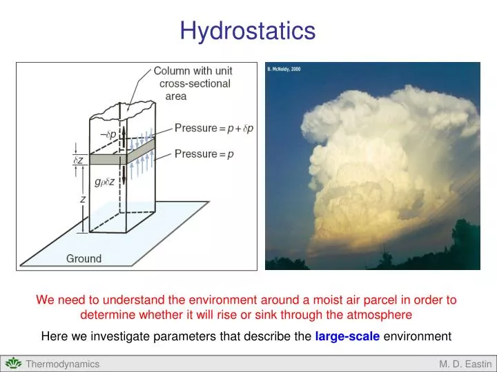
Hydrostatics We need to understand the environment around a moist air parcel in order to determine whether it will rise or sink through the atmosphere Here we investigate parameters that describe the large-scale environment M. D. Eastin
Hydrostatics • Outline: • Review of the Atmospheric Vertical Structure • Hydrostatic Equation • Geopotential Height • Application • Hypsometric Equation • Applications • Layer Thickness • Heights of Isobaric Surfaces • Reduction of Surface Pressure to Sea Level M. D. Eastin
Review of Atmospheric Vertical Structure • Pressure: • Measures the force per unit area exerted • by the weight of all the moist air lying • above that height • Decreases with increasing height • Density: • Mass per unit volume • Decreases with increasing height • Temperature (or Virtual Temperature): • Related to density and pressure via the • Ideal Gas Law for moist air • Decreases with increasing height z(km) Tropopause 12 Tv(K) p(mb) 0 -60 200 15 1013 M. D. Eastin
Hydrostatic Equation • Balance of Forces: • Consider a vertical column of air • The mass of air between heights z and • z+dz is ρdz and defines a slab of air • in the atmosphere • The downward force acting on this slab • is due to the mass of the air above and • gravity (g) pulling the mass downward • The upward force acting on this slab is • due to the change in pressure through • the slab M. D. Eastin
Hydrostatic Equation • Balance of Forces: • The upward and downward forces must • balance (Newton’s laws) • Simply re-arrange and we arrive at the • hydrostatic equation: M. D. Eastin
Hydrostatic Equation • Application: • Represents a balanced state between the downward directed • gravitational force and the upward directed pressure gradient force • Valid for large horizontal scales (> 1000 km; synoptic) in our atmosphere • Implies no vertical motion occurs on these large scales • The large-scale environment of a moist air parcel • is in hydrostatic balance and does not move up or down • Note: Hydrostatic balance is NOT valid for small horizontal scales (i.e. the • moist air parcel moving through a thunderstorm) M. D. Eastin
Geopotential Height • Definition: • The geopotential (Φ) at any point in the Earth’s atmosphere is the amount of • work that must be done against the gravitational field to raise a mass of 1 kg • from sea-level to that height. • Accounts for the change in gravity (g) with height Height Gravity z (km) g (m s-2) 0 9.81 1 9.80 10 9.77 100 9.50 M. D. Eastin
Geopotential Height • Definition: • The geopotential height (Z) is the actual height normalized by the globally • averaged acceleration due to gravity at the Earth’s surface (g0 = 9.81 m s-2), • and is defined by: • Used as the vertical coordinate in most atmospheric applications in which • energy plays an important role (i.e. just about everything) • Lucky for us → g ≈ g0 in the troposphere Height Geopotential Height Gravity z (km) Z (km) g (m s-2) 0 0.00 9.81 1 1.00 9.80 10 9.99 9.77 100 98.47 9.50 M. D. Eastin
Geopotential Height • Application: • The geopotential height (Z) is the standard “height” parameter plotted on • isobaric charts constructed from daily soundings: 500 mb Geopotential heights (Z) are solid black contours (Ex: Z = 5790 meters) Air temperatures (T) are red dashed contours (Ex: T = -11ºC) Winds are shown as barbs M. D. Eastin
Hypsometric Equation • Derivation: • If we combine the Hydrostatic Equation with the Ideal Gas Law for moist air • and the Geopotential Height, we can derive an equation that defines the • thickness of a layer between two pressure levels in the atmosphere • 1. Substitute the ideal gas law into the Hydrostatic Equation M. D. Eastin
Hypsometric Equation Derivation: 2. Re-arranging the equation and using the definition of geopotenital height: 3. Integrate this equation between two geopotential heights (Φ1 and Φ2) and the two corresponding pressures (p1 and p2), assuming Tv is constant in the layer M. D. Eastin
Hypsometric Equation Derivation: 4. Performing the integration: 5. Dividing both sides by the gravitational acceleration at the surface (g0): M. D. Eastin
Hypsometric Equation • Derivation: • 6. Using the definition of geopotential height: • Defines the geopotential thickness (Z2 – Z1) between any two pressure levels (p1 and p2) in the atmosphere. Hypsometric Equation M. D. Eastin
Hypsometric Equation • Interpretation: • The thickness of a layer between two pressure levels is proportional to the • mean virtual temperature of that layer. • If Tv increases, the air between the • two pressure levels expands and • the layer becomes thicker • If Tv decreases, the air between the • two pressure levels compresses • and the layer becomes thinner Black solid lines are pressure surfaces Hurricane (warm core) Mid-latitude Low (cold core) M. D. Eastin
Hypsometric Equation Interpretation: p2 +Z Layer 1: p1 +Z p2 Layer 2: p1 Which layer has the warmest mean virtual temperature? M. D. Eastin
Hypsometric Equation Application: Computing the Thickness of a Layer A sounding balloon launched last week at Greensboro, NC measured a mean temperature of 10ºC and a mean specific humidity of 6.0 g/kg between the 700 and 500 mb pressure levels. What is the geopotential thickness between these two pressure levels? T = 10ºC = 283 K q = 6.0 g/kg = 0.006 p1 = 700 mb p2 = 500 mb g0 = 9.81 m/s2 Rd = 287 J /kg K 1. Compute the mean Tv → Tv = 284.16 K 2. Compute the layer thickness (Z2 – Z1) → Z2 – Z1 = 2797.2 m M. D. Eastin
Hypsometric Equation Application: Computing the Height of a Pressure Surface Last week the surface pressure measured at the Charlotte airport was 1024 mb with a mean temperature and specific humidity of 21ºC and 11 g/kg, respectively, below cloud base. Calculate the geopotential height of the 1000 mb pressure surface. T = 21ºC = 294 K q = 11.0 g/kg = 0.011 p1 = 1024 mb p2 = 1000 mb Z1 = 0 m (at the surface) Z2 = ??? g0 = 9.81 m/s2 Rd = 287 J /kg K 1. Compute the mean Tv → Tv = 295.97 K 2. Compute the height of 1000 mb (Z2) → Z2 = 198.9 m M. D. Eastin
400 mb 500 mb Kathmandu 600 mb 700 mb Aspen 850 mb Denver Hypsometric Equation • Application: Reduction of Pressure to Sea Level • In mountainous regions, the difference in surface pressure from one observing • station to the next is largely due to elevation changes • In weather forecasting, we need to isolate that part of the pressure field that • is due to the passage of weather systems (i.e., “Highs” and “Lows”) • We do this by adjusting all observed surface pressures (psfc) to a common • reference level → sea level (where Z = 0 m) M. D. Eastin
Hypsometric Equation Application: Reduction of Pressure to Sea Level Last week the surface pressure measured in Asheville, NC was 934 mb with a surface temperature and specific humidity of 14ºC and 8 g/kg, respectively. If the elevation of Asheville is 650 meters above sea level, compute the surface pressure reduced to sea level. T = 14ºC = 287 K q = 8.0 g/kg = 0.008 p1 = ??? (at sea level) p2 = 934 mb (at ground level) Z1 = 0 m (sea level) Z2 = 650 m (ground elevation) g0 = 9.81 m/s2 Rd = 287 J /kg K 1. Compute the surface Tv → Tv = 288.40 K 2.Solve the hypsometric equation for p1 (at sea level) 3. Compute the sea level pressure (p1) → p1 = 1009 mb M. D. Eastin
Hypsometric Equation • Application: Reduction of Pressure to Sea Level • All pressures plotted on surface weather maps have been “reduced to sea level” M. D. Eastin
In Class Activity Layer Thickness: Observations from yesterday’s Charleston, SC sounding: Pressure (mb) Temperature (ºC) Specific Humidity (g/kg) 850 10.4 9.2 700 1.8 3.5 Compute the thickness of the 850-700 mb layer Reduction of Pressure to Sea Level: Observations from the Charlotte Airport: Z = 237 m (elevation above sea level) p = 983 mb T = 10.5ºC q = 15.6 g/kg Compute the surface pressure reduced to sea level Write your answers on a sheet of paper and turn in by the end of class… M. D. Eastin
Hydrostatics • Summary: • Review of the Atmospheric Vertical Structure • Hydrostatic Equation • Geopotential Height • Application • Hypsometric Equation • Applications • Layer Thickness • Heights of Isobaric Surfaces • Reduction of Surface Pressure to Sea Level M. D. Eastin
References Houze, R. A. Jr., 1993: Cloud Dynamics, Academic Press, New York, 573 pp. Markowski, P. M., and Y. Richardson, 2010: Mesoscale Meteorology in Midlatitudes, Wiley Publishing, 397 pp. Petty, G. W., 2008: A First Course in Atmospheric Thermodynamics, Sundog Publishing, 336 pp. Tsonis, A. A., 2007: An Introduction to Atmospheric Thermodynamics, Cambridge Press, 197 pp. Wallace, J. M., and P. V. Hobbs, 1977: Atmospheric Science: An Introductory Survey, Academic Press, New York, 467 pp. M. D. Eastin