Download
1 / 51
510 likes | 737 Vues
GEOGG121: Methods Differential Equations. Dr. Mathias (Mat) Disney UCL Geography Office: 113, Pearson Building Tel: 7670 0592 Email: mdisney@ucl.geog.ac.uk www.geog.ucl.ac.uk /~ mdisney. Lecture outline. Differential equations Introduction & importance Types of DE Examples

E N D
GEOGG121: MethodsDifferential Equations Dr. Mathias (Mat) Disney UCL Geography Office: 113, Pearson Building Tel: 7670 0592 Email: mdisney@ucl.geog.ac.uk www.geog.ucl.ac.uk/~mdisney
Lecture outline • Differential equations • Introduction & importance • Types of DE • Examples • Solving ODEs • Analytical methods • General solution, particular solutions • Separation of variables, integrating factors,linear operators • Numerical methods • Euler, Runge-Kutta • V. short intro to Monte Carlo (MC) methods
Reading material • Textbooks These are good UG textbooks that have WAY more detail than we need • Boas, M. L., 1985 (2nd ed) Mathematical Methods in the Physical Sciences, Wiley, 793pp. • Riley, K. F., M. Hobson & S. Bence (2006) Mathematical Methods for Physics & Engineering, 3rd ed., CUP. • Croft, A., Davison, R. & Hargreaves, M. (1996) Engineering Mathematics, 2nd ed., Addison Wesley. • Methods, applications • Wainwright, J. and M. Mulligan (eds, 2004) Environmental Modelling: Finding Simplicity in Complexity, J. Wiley and Sons, Chichester. Lots of examples particularly hydrology, soils, veg, climate. Useful intro. ch 1 on models and methods • Campbell, G. S. and J. Norman (1998) An Introduction to Environmental Biophysics, Springer NY, 2nd ed. Excellent on applications eg Beer’s Law, heat transport etc. • Monteith, J. L. and M. H. Unsworth(1990) Principles of Environmental Physics, Edward Arnold. Small, but wide-ranging and superbly written. • Links • http://www.math.ust.hk/~machas/differential-equations.pdf • http://www.physics.ohio-state.edu/~physedu/mapletutorial/tutorials/diff_eqs/intro.html
Introduction • What is a differential equation? • General 1st order DEs • 1st case t is independent variable, x is dependent variable • 2nd case, x is independent variable, y dependent • Extremely important • Equation relating rate of change of something (y) wrt to something else (x) • Any dynamic system (undergoing change) may be amenable to description by differential equations • Being able to formulate & solve is incredibly powerful
Examples • Velocity • Change of distance x with time t i.e. • Acceleration • Change of v with t i.e. • Newton’s 2nd law • Net force on a particle = rate of change of linear momentum (m constant so… • Harmonic oscillator • Restoring force F on a system displacement (-x) i.e. • So taking these two eqns we have
Examples • Radioactive decay of unstable nucleus • Random, independent events, so for given sample of N atoms, no. of decay events –dN in time dt N • So N(t) depends on No (initial N) and rate of decay • Beer’s Law – attenuation of radiation • For absorption only (no scattering), decreases in intensity (flux density) of radiation at some distance x into medium, Φ(x) is proportional to x • Same form as above – will see leads to exponential decay • Radiation in vegetation, clouds etcetc
Examples • Compound Interest • How does an investment S(t), change with time, given an annual interest rate r compounded every time interval Δt, and annual deposit amount k? • Assuming deposit made after every time interval Δt • So as Δt0
Examples • Population dynamics • Logistic equation (Malthus, Verhulst, Lotka….) • Rate of change of population P with t depends on Po, growth rate r (birth rate – death rate) & max available population or ‘carrying capacity’ K • P << K, dP/dt rP but as P increases (asymptotically) to K, dP/dtgoes to 0 (competition for resources – one in one out!) • For constant K, if we set x = P/K then http://www.scholarpedia.org/article/Predator-prey_model#Lotka-Volterra_Model
Examples • Population dynamics: II • Lotka-Volterra (predator-prey) equations • Same form, butnow two populations x and y, with time – • y is predator and yt+1 depends on yt AND prey population (x) • x is prey, and xt+1 depends on xt AND y • a, b, c, d – parameters describing relationship of y to x • More generally can describe • Competition – eg economic modelling • Resources – reaction-diffusion equations
Examples • Transport: momentum, heat, mass…. • Transport usually some constant (proportionality factor) x driving force • Newton’s Law of viscosity for momentum transport • Shear stress, τ, between fluid layers moving at different speeds - velocity gradient perpendicular to flow, μ = coeff. of viscosity • Fourier’s Law of heat transport • Heat flux density H in a material is proportional to (-) T gradient and area perpendicular to gradient through which heat flowing, k = conductivity. In 1D case… • Fick’s Law of diffusive transport • Flux density F’j of a diffusing substance with molecular diffusivity Dj across density gradient dρj/dz (j is for different substances that diffuse through air) • See Campbell and Norman chapter 6
Types: analytical, non-analytical • Analytical, closed form • Exact solution e.g. in terms of elementary functions such as ex, log x, sin x • Non-analytical • No simple solution in terms of basic functions • Solution requires numerical methods (iterative) to solve • Provide an approximate solution, usually as infinite series
Types: analytical, non-analytical • Analytical example • Exact solution e.g. • Solve by integrating both sides • This is a GENERAL solution • Contains unknown constants • We usually want a PARTICULAR solution • Constants known • Requires BOUNDARY conditions to be specified
Types: analytical, non-analytical • Particular solution? • BOUNDARY conditions e.g.set t = 0 to get c1, 2 i.e. • So x0 is the initial value and we have • Exponential model ALWAYS when dx/dt x • If a>0 == growth; if a < 0 == decay • Population: a = growth rate i.e. (births-deaths) • Beer’s Law: a = attenuation coeff. (amount x absorp. per unit mass) • Radioactive decay: a = decay rate
Types: analytical, non-analytical • Analytical: population growth/decay example Log scale – obviously linear….
Types: ODEs, PDEs • ODE (ordinary DE) • Contains only ordinary derivatives • PDE (partial DE) • Contains partial derivatives – usually case when depends on 2 or more independent variables • E.g. wave equation: displacement u, as function of time, t and position x
Types: Order • ODE (ordinary DE) • Contains only ordinary derivatives (no partials) • Can be of different order • Order of highest derivative 2nd 1st 2nd
Types: Order -> Degree • ODE (ordinary DE) • Can further subdivide into different degree • Degree (power) to which highest order derivative raised 1st order 3rd degree 1st order 1st degree 2nd order 2nd degree
Types: Linearity • ODE (ordinary DE) • Linear or non-linear? • Linear if dependent variable and all its derivatives occur only to the first power, otherwise, non-linear • Product of terms with dependent variable == non-linear • Functions sin, cos, exp, ln also non-linear Non-linear ydy/dx Non-linear y2 term Non-linear sin y term Linear
Solving • General solution • Often many solutions can satisfy a differential eqn • General solution includes all these e.g. • Verify that y = Cex is a solution of dy/dx = y, C is any constant • So • And for all values of x, and eqn is satisfied for any C • C is arbitrary constant, vary it and get all possible solutions • So in fact y = Cex is the general solution of dy/dx = y
Solving • But for a particular solution • We must specify boundary conditions • Eg if at x = 0, we know y = 4 then from general solution • 4 = Ce0 so C = 4 and • is the particular solution of dy/dx = y that satisfies the condition that y(0) = 4 • Can be more than one constant in general solution • For particular solution number of given independent conditions MUST be same as number of constants
Types: analytical, non-analytical • Analytical: Beer’s Law - attenuation • k is extinction coefficient – absorptivity per unit depth, z (m-1) • E.g. attenuation through atmosphere, where path length (z) 1/cos(θsun), θsun is the solar zenith angle • Take logs: • Plot z against ln(ϕ), slope is k, intercept is ϕ0 i.e. solar radiation with no attenuation (top of atmos. – solar constant) • [NB taking logs v powerful – always linearise if you can!]
Initial & boundary conditions • One point conditions • We saw as general solution of • Need 2 conditions to get particular solution • May be at a single point e.g. x = 0, y = 0 and dy/dx = 1 • So and solution becomes • Now apply second condition i.e. dy/dx = 1 when x = 0 so differentiate • Particular solution is then
Solving: examples • Verify that satisfies • Verify that is a solution of • (2nd order, 1st degree, linear)
Initial & boundary conditions • Two point conditions • Again consider • Solution satisfying y = 0 when x = 0 AND y = 1 when x = 3π/2 • So apply first condition to general solution • i.e. and solution is • Applying second condition we see • And B = -1, so the particular solution is • If solution required over interval a ≤ x ≤ b and conditions given at both ends, these are boundary conditions (boundary value problem) • Solution subject to initial conditions = initial value problem
Separation of variables • We have considered simple cases so far • Where and so • What about cases with ind. & dep. variables on RHS? • E.g. • Important class of separable equations. Div by g(y) to solve • And then integrate both sides wrt x
Separation of variables • Equation is now separated & if we can integ. we have y in terms of x • Eg where and • So multiply both sides by y to give and then integrate both sides wrt x • i.e. and so and • If we define D = 2C then Eg See Croft, Davison, Hargreaves section 18, or http://www.cse.salford.ac.uk/profiles/gsmcdonald/H-Tutorials/ordinary-differential-equations-separation-variables.pdf http://en.wikipedia.org/wiki/Separation_of_variables
Using an integrating factor • For equations of form • Where P(x) and Q(x) are first order linear functions of x, we can multiply by some (as yet unknown) function of x, μ(x) • But in such a way that LHS can be written as • And then • Which is said to be exact, with μ(x) as the integrating factor • Why is this useful? Eg See Croft, Davison, Hargreaves section 18, or http://www.cse.salford.ac.uk/profiles/gsmcdonald/H-Tutorials/ordinary-differential-equations-integrating-factor.pdfhttp://en.wikipedia.org/wiki/Integrating_factor
Using an integrating factor • Because it follows that • And if we can evaluate the integral, we can determine y • So as above, we want • Use product rule i.e. and so, from above • and by inspection we can see that • This is separable (hurrah!) i.e. http://en.wikipedia.org/wiki/Product_rulehttp://www.cse.salford.ac.uk/profiles/gsmcdonald/H-Tutorials/ordinary-differential-equations-integrating-factor.pdf
Using an integrating factor • And we see that (-lnK is const. of integ.) • And so • We can choose K = 1 (as we are multiplying all terms in equation by integ. factor it is irrelevant), so • Integrating factor for is given by • And solution is given by http://en.wikipedia.org/wiki/Product_rulehttp://www.cse.salford.ac.uk/profiles/gsmcdonald/H-Tutorials/ordinary-differential-equations-integrating-factor.pdf
Using an integrating factor: example • Solve • From previous we see that and • Using the formula above • And we know the solution is given by • So , as
2nd order linear equations • Form • Where p(x), q(x), r(x) and f(x) are fns of x only • This is inhomogeneous(depon y) • Related homogeneousform ignoring term independent of y • Use shorthand L{y} when referring to general linear diff. eqn to stand for all terms involving y or its derivatives. From above • for inhomogeneous general case • And for general homogenous case • Eg if then where
Linear operators • When L{y} = f(x) is a linear differential equation, L is a linear differential operator • Any linear operator L carries out an operation on functions f1 and f2 as follows • where a is a constant • where a, b are constants • Example: if show that • and
Linear operators • Note that L{y} = f(x) is a linear diff. eqn so L is a linear diff operator • So • we see • And rearrange: • & because differentiation is a linear operator we can now see • For the second case • So
Partial differential equations • DEs with two or more dependent variables • Particularly important for motion (in 2 or 3D), where eg position (x, y, z) varying with time t • Key example of wave equation • Eg in 1D where displacement u depends on time and position • For speed c, satisfies • Show is a solution of • Calculate partial derivatives of u(x, t) wrt to x, then t i.e.
Partial differential equations • Now 2nd partial derivatives of u(x, t) wrt to x, then t i.e. • So now • More generally we can express the periodic solutions as (remembering trig identities) • and • Where k is the wave vector (2π/λ); ω is the angular frequency (rads s-1) = 2π/T for period T; http://en.wikipedia.org/wiki/List_of_trigonometric_identities http://www.physics.usu.edu/riffe/3750/Lecture%2018.pdf http://en.wikipedia.org/wiki/Wave_vector
Partial differential equations • In 3D? • Just consider y and z also, so for q(x, y, z, t) • Some v. important linear differential operators • Del (gradient operator) • Del squared (Laplacian) • Lead to eg Maxwell’s equations http://www.physics.usu.edu/riffe/3750/Lecture%2018.pdf
Numerical approaches • Euler’s Method • Consider 1st order eqn with initial cond. y(x0) = y0 • Find an approx. solution yn at equally spaced discrete values (steps) of x, xn • Euler’s method == find gradient at x = x0 i.e. • Tangent line approximation True solution y y(x1) Tangent approx. y1 y0 Croft et al., p495 Numerical Recipes in C ch. 16, p710 http://apps.nrbook.com/c/index.html x0 x1 0 x http://en.wikipedia.org/wiki/Numerical_ordinary_differential_equations
Numerical approaches • Euler’s Method • True soln passes thru (x0, y0) with gradient f(x0, y0) at that point • Straight line (y = mx + c) approx has eqn • This approximates true solution but only near (x0, y0), so only extend it short dist. h along x axis to x = x1 • Here, y = y1 and • Since h = x1-x0 we see • Can then find y1, and we then know (x1, y1)…..rinse, repeat…. True solution y y(x1) Tangent approx. y1 y0 Generate series of values iteratively Accuracy depends on h Croft et al., p495 Numerical Recipes in C ch. 16, p710 http://apps.nrbook.com/c/index.html x0 x1 0 x
Numerical approaches • Euler’s Method: example • Use Euler’s method with h = 0.25 to obtain numerical soln. of with y(0) = 2, giving approx. values of y for 0 ≤ x ≤ 1 • Need y1-4 over x1 = 0.25, x2 = 0.5, x3 = 0.75, x4 = 1.0 say, so • with x0 = 0 y0 = 2 • And NB There are more accurate variants of Euler’s method.. Exercise: this can be solved ANALYTICALLY via separation of variables. What is the difference to the approx. solution?
Numerical approaches • Runge-Kutta methods (4th order here….) • Family of methods for solving DEs (Euler methods are subset) • Iterative, starting from yi, no functions other than f(x,y) needed • No extra differentiation or additional starting values needed • BUT f(x, y) is evaluated several times for each step • Solve subject to y = y0 when x = x0, use • where Euler Croft et al., p502 Rile et al. p1026 Numerical Recipes in C ch. 16, p710 http://apps.nrbook.com/c/index.html http://en.wikipedia.org/wiki/Numerical_ordinary_differential_equations http://en.wikipedia.org/wiki/Runge%E2%80%93Kutta_methods
Numerical approaches • Runge-Kutta example • As before, but now use R-K with h = 0.25 to obtain numerical soln. of with y(0) = 2, giving approx. values of y for 0 ≤ x ≤ 1 • So for i = 0, first iteration requires • And finally • Repeat! c.f. 2 from Euler, and 1.8824 from analytical
Very brief intro to Monte Carlo • Brute force method(s) for integration / parameter estimation / sampling • Powerful BUT essentially last resort as involves random sampling of parameter space • Time consuming – more samples gives better approximation • Errors tend to reduce as 1/N1/2 • N = 100 -> error down by 10; N = 1000000 -> error down by 1000 • Fast computers can solve complex problems • Applications: • Numerical integration (eg radiative transfer eqn), Bayesian inference, computational physics, sensitivity analysis etcetc Numerical Recipes in C ch. 7, p304 http://apps.nrbook.com/c/index.html http://en.wikipedia.org/wiki/Monte_Carlo_method http://en.wikipedia.org/wiki/Monte_Carlo_integration
Basics: MC integration • Pick N random points in a multidimensional volume V, x1, x2, …. xN • MC integration approximates integral of function f over volume V as • Where and • +/- term is 1SD error – falls of as 1/N1/2 Choose random points in A Integral is fraction of points under curve x A From http://apps.nrbook.com/c/index.html
Basics: MC integration • Why not choose a grid? Error falls as N-1 (quadrature approach) • BUT we need to choose grid spacing. For random we sample until we have ‘good enough’ approximation • Is there a middle ground? Pick points sort of at random BUT in such a way as to fill space more quickly (avoid local clustering)? • Yes – quasi-random sampling: • Space filling: i.e. “maximally avoiding of each other” FROM: http://en.wikipedia.org/wiki/Low-discrepancy_sequence Sobol method v pseudorandom: 1000 points
Summary • Differential equations • Describe dynamic systems – wide range of examples, particularly motion, population, decay (radiation – Beer’s Law, mass – radioactivity) • Types • Analytical, closed form solution, simple functions • Non-analytical: no simple solution, approximations? • ODEs, PDEs • Order: highest power of derivative • Degree: power to which highest order derivative is raised • Linear/non: • Linear if dependent variable and all its derivatives occur only to the first power, otherwise, non-linear
Summary • Solving • Analytical methods? • Find general solution by integrating, leaves constants of integration • To find a particular solution: need boundary conditions (initial, ….) • Integrating factors, linear operators • Numerical methods? • Euler, Runge-Kutta – find approx. solution for discrete points • Monte Carlo methods • Very useful brute force numerical approach to integration, parameter estimation, sampling • If all else fails, guess…..
Example • Radioactive decay • Random, independent events, so for given sample of N atoms, no. of decay events –dN in time dt N so • Where λ is decay constant (analogous to Beer’s Law k) units 1/t • Solve as for Beer’s Law case so • i.e. N(t) depends on No (initial N) and rate of decay • λ often represented as 1/tau, where tau is time constant – mean lifetime of decaying atoms • Half life (t=T1/2) = time taken to decay to half initial N i.e. N0/2 • Express T1/2 in terms of tau
Example • Radioactive decay • EG: 14C has half-life of 5730 years & decay rate = 14 per minute per gram of natural C • How old is a sample with a decay rate of 4 per minute per gram? • A: N/N0 = 4/14 = 0.286 • From prev., tau = T1/2/ln2 = 5730/ln2 = 8267 yrs • So t = -tau x ln(N/N0) = 10356 yrs
Exercises • General solution of is given by • Find particular solution satisfies x = 3 and dx/dt = 5 when t =0 • Resistor (R) capacitor (L) circuit (p458, Croft et al), with current flow i(t) described by • Use integrating factor to find i(t)….approach: re-write as