Download

1 / 54
540 likes | 635 Vues
GEOGG121: Methods Inversion I : linear approaches. Dr. Mathias (Mat) Disney UCL Geography Office: 113, Pearson Building Tel: 7670 0592 Email: mdisney@ucl.geog.ac.uk www.geog.ucl.ac.uk /~ mdisney. Lecture outline. Linear models and inversion Least squares revisited, examples

E N D
GEOGG121: MethodsInversion I: linear approaches Dr. Mathias (Mat) Disney UCL Geography Office: 113, Pearson Building Tel: 7670 0592 Email: mdisney@ucl.geog.ac.uk www.geog.ucl.ac.uk/~mdisney
Lecture outline • Linear models and inversion • Least squares revisited, examples • Parameter estimation, uncertainty • Practical examples • Spectral linear mixture models • Kernel-driven BRDF models and change detection
Reading • Linear models and inversion • Linear modelling notes: Lewis, 2010 • Chapter 2 of Press et al. (1992) Numerical Recipes in C (online version http://apps.nrbook.com/c/index.html) • http://en.wikipedia.org/wiki/Linear_model • http://en.wikipedia.org/wiki/System_of_linear_equations
Linear Models • For some set of independent variables x = {x0, x1, x2, … , xn} have a model of a dependent variable y which can be expressed as a linear combination of the independent variables.
Linear Mixture Modelling • Spectral mixture modelling: • Proportionate mixture of (n) end-member spectra • First-order model: no interactions between components Constraint
Linear Mixture Modelling • r = {rl0, rl1, … rlm, 1.0} • Measured reflectance spectrum (m wavelengths) • nx(m+1) matrix:
Linear Mixture Modelling • n=(m+1) – square matrix • Eg n=2 (wavebands), m=2 (end-members)
r1 r2 Reflectance Band 2 r r3 Reflectance Band 1
Linear Mixture Modelling • as described, is not robust to error in measurement or end-member spectra; • Proportions must be constrained to lie in the interval (0,1) • - effectively a convex hull constraint; • m+1 end-member spectra can be considered; • needs prior definition of end-member spectra; cannot directly take into account any variation in component reflectances • e.g. due to topographic effects
Linear Mixture Modelling in the presence of Noise • Define residual vector • minimise the sum of the squares of the error e, i.e. Method of Least Squares (MLS)
Error Minimisation • Set (partial) derivatives to zero
Error Minimisation • Can write as: Solve for P by matrix inversion
x x1 x2 y x
Weight of Determination (1/w) • Calculate uncertainty at y(x)
P1 RMSE P0
P1 RMSE P0
Issues • Parameter transformation and bounding • Weighting of the error function • Using additional information • Scaling
Parameter transformation and bounding • Issue of variable sensitivity • E.g. saturation of LAI effects • Reduce by transformation • Approximately linearise parameters • Need to consider ‘average’ effects
Weighting of the error function • Different wavelengths/angles have different sensitivity to parameters • Previously, weighted all equally • Equivalent to assuming ‘noise’ equal for all observations
Weighting of the error function • Can ‘target’ sensitivity • E.g. to chlorophyll concentration • Use derivative weighting (Privette 1994)
Using additional information • Typically, for Vegetation, use canopy growth model • See Moulin et al. (1998) • Provides expectation of (e.g.) LAI • Need: • planting date • Daily mean temperature • Varietal information (?) • Use in various ways • Reduce parameter search space • Expectations of coupling between parameters
Scaling • Many parameters scale approximately linearly • E.g. cover, albedo, fAPAR • Many do not • E.g. LAI • Need to (at least) understand impact of scaling
Linear Kernel-driven Modelling of Canopy Reflectance • Semi-empirical models to deal with BRDF effects • Originally due to Roujean et al (1992) • Also Wanner et al (1995) • Practical use in MODIS products • BRDF effects from wide FOV sensors • MODIS, AVHRR, VEGETATION, MERIS
Satellite, Day 1 Satellite, Day 2 X
Model parameters: Isotropic Volumetric Geometric-Optics Linear BRDF Model • of form:
Model Kernels: Volumetric Geometric-Optics Linear BRDF Model • of form:
Volumetric Scattering • Develop from RT theory • Spherical LAD • Lambertian soil • Leaf reflectance = transmittance • First order scattering • Multiple scattering assumed isotropic
Volumetric Scattering • If LAI small:
Similar approach for RossThick Volumetric Scattering • Write as: RossThin kernel
Geometric Optics • Consider shadowing/protrusion from spheroid on stick (Li-Strahler 1985)
Geometric Optics • Assume ground and crown brightness equal • Fix ‘shape’ parameters • Linearised model • LiSparse • LiDense
Retro reflection (‘hot spot’) Kernels Volumetric (RossThick) and Geometric (LiSparse) kernels for viewing angle of 45 degrees
Kernel Models • Consider proportionate (a) mixture of two scattering effects
Using Linear BRDF Models for angular normalisation • Account for BRDF variation • Absolutely vital for compositing samples over time (w. different view/sun angles) • BUT BRDF is source of info. too! MODIS NBAR (Nadir-BRDF Adjusted Reflectance MOD43, MCD43) http://www-modis.bu.edu/brdf/userguide/intro.html
MODIS NBAR (Nadir-BRDF Adjusted Reflectance MOD43, MCD43) http://www-modis.bu.edu/brdf/userguide/intro.html
And uncertainty via BRDF Normalisation • Fit observations to model • Output predicted reflectance at standardised angles • E.g. nadir reflectance, nadir illumination • Typically not stable • E.g. nadir reflectance, SZA at local mean
Linear BRDF Models to track change 220 days of Terra (blue) and Aqua (red) sampling over point in Australia, w. sza (T: orange; A: cyan). • Examine change due to burn (MODIS) Time series of NIR samples from above sampling FROM: http://modis-fire.umd.edu/Documents/atbd_mod14.pdf
MODIS Channel 5 Observation DOY 275
MODIS Channel 5 Observation DOY 277
Detect Change • Need to model BRDF effects • Define measure of dis-association
MODIS Channel 5 Prediction DOY 277
MODIS Channel 5 Discrepancy DOY 277
MODIS Channel 5 Observation DOY 275
MODIS Channel 5 Prediction DOY 277
MODIS Channel 5 Observation DOY 277