Download
1 / 23
230 likes | 242 Vues
In summary. We use this in Ch. 10. [ r ] = dEG n /2 p,. . Where G = [EI – H - S ] -1 , [A] = G G G +. , G n = G S in G +. . . . We will use this in this Chapter. . . . . . . . . Already used in Chapter 1. g 1 f 1 + g 2 f 2. . . N = dE D(E-U).

E N D
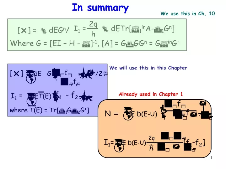
In summary We use this in Ch. 10 [r] = dEGn/2p, Where G = [EI – H - S]-1, [A] = GGG+ , Gn = GSinG+ We will use this in this Chapter Already used in Chapter 1 g1f1 +g2f2 N = dE D(E-U) f1 - f2 g1f1 +g2f2 I1=dET(E) [r]= dE G G+/2p g1 + g2 2q g1g2 I1 = dETr[S1inA-G1Gn] h g1 + g2 2q I1= dE D(E-U)[f1-f2] h where T(E) = Tr[G1GG2G+]
Onto practical applications f1 - f2 g1f1 +g2f2 I1=dET(E) [r]= dE G G+/2p where T(E) = Tr[G1GG2G+] What do these equations predict for coherent quantum transport?
G1(1,1) = ħv1/a, G2(N,N) = ħv2/a 1-D wire -t e0 v2 v1 {y} = [G]{S} Only S(1) exists, equal to iħv1/a t = y(N) = G(N,1)S(1) T = |t|2v2/v1 = (ħv1/a)(ħv2/a)|G(1,N)|2 Thus T = Tr[G1GG2G+]
1-D wire -t e0 What do we expect for DOS, Transmission ? H = e0 S1 = S2 = -teika G1 = i(S1-S1+)= 2tsinka = G2 = G/2 G = (EI-H-S1-S2)-1 = 1/(E-e0+2teika) E = e0 - 2tcoska ħv = dE/dk = 2tasinka G = (EI-H-S1-S2)-1 = i/2tsinka D = GGG+/2p = 1/2ptsinka = a/pħv T = G1GG2G+ = 1
1-D wire Like Exam 2
1-D wire EXPT Halbritter PRB ’04
1-D wire with weak coupling to contacts -t e0 v2 v1 S1(1,1) = S2(N,N) = -[t’2/t]eika t’ < t isolates wire and makes its levels discrete (‘molecule’) Discrete levels create quantum resonances (standing waves between ends)
1-D wire with weak coupling to contacts Ignoring Laplace term (‘screening’)
Reed 1-D wire with weak coupling to contacts
1-D wire with a defect -t e0 e1 H = e1 S1 = S2 = -teika G1 = i(S1-S1+)= 2tsinka = G2 = G/2 G = (EI-H-S1-S2)-1 = 1/(e0-e1-2itsinka) E = e0 - 2tcoska ħv = dE/dk = 2tasinka G = (EI-H-S1-S2)-1 D = GGG+/2p = ħv/p[ħ2v2 + (De)2] T = G1GG2G+ = 1/[1 + (De/ħv)2]
Analytical Derivation -t e0 e1 y|+ - y|- = 0 t-(1+r) = 0 dy/dz|+ - dy/dz|- = [2mU0/ħ2]y|0 ik[t-(1-r)] = 2mU0t/ħ2 T = |t|2 = ħ2v2/(ħ2v2+U02)
Defect, e0-e1=2 T < 1 More importantly, split off level outside band (that’s how dopants work!)
e0 -t 0 0 Hon = Hoff = e0 -t t 0 g-1 = a – bgb+, a = EI-Hon, b = -Hoff S1 = S2 = bgb+ 1-D wire with a basis -t e0
2-D wire e0 0 -t -t Hon = Hoff = e0 -t 0 -t g-1 = a – bgb+, a = EI-Hon, b = -Hoff S1 = S2 = bgb+ e0 -t e0 -t
Multiple Modes EI = Hon – Hoffeika – Hoff+e-ika Bands E1 = 2t(1-coska)+t, E2=2t(1-coska)-t
2-D wire e0 -t e0 -t g-1 = a – bgb+, a = EI-Hon, b = -Hoff S1 = S2 = bgb+
Multiple Modes Bands E1 = 2t(1-coska)-2t, E2,3 = 2t(1-coska)+t
1-D wire with a barrier -t e0
1-D wire with a barrier -t e0 Slight subtleties – 2D cross section sum over transverse modes (f F)
gd=0.1 ech=0 ed=0.5 t= 1 EF=-0.5 g0ch = 1/(EF-ech + igch) g0d = 1/(EF-ed + qVG + igd) 1-D wire with a scatterer g-1ch = (g0ch)-1 – t2g0d Dch = i(gch-gch+)/(2p)
Fano interference between a channel and a quantum dot 1-D wire with a scatterer