Download
1 / 87
900 likes | 930 Vues
Front-end Electronics and Signal Processing - I. Politecnico di Milano, Dipartimento di Elettronica e Informazione, and INFN, Sezione di Milano Chiara.Guazzoni@mi.infn.it http://www.elet.polimi.it/upload/guazzoni. Table of Contents – Part I. Introduction

E N D
Front-end Electronics and Signal Processing- I Politecnico di Milano, Dipartimento di Elettronica e Informazione, and INFN, Sezione di Milano Chiara.Guazzoni@mi.infn.it http://www.elet.polimi.it/upload/guazzoni C. Guazzoni – II Regional ICFA Instrumentation School – Istanbul, September 2, 2005
Table of Contents – Part I • Introduction • Signal formation and Ramo’s theorem • Noise analysis and noise modeling in electronic devices • Basic blocks in a detection system • Equivalent noise charge concept and calculation • Capacitive matching • Time measurements • Time-variant filters C. Guazzoni – II Regional ICFA Instrumentation School – Istanbul, September 2, 2005
Introduction – I Detector signal processing is the set of operations to be performed on the current pulse delivered by the detector in order to extract the information about: • The energy released by the radiation in the sensitive volume of the detector spectroscopy measurements • The time of occurrenceof the interaction timing measurements • The position where, in a segmented detector, the radiation hits its sensitive volume imaging In the following we will limit our attention to capacitive detectors (the large majority, however…) C. Guazzoni – II Regional ICFA Instrumentation School – Istanbul, September 2, 2005
Introduction – II Parameters to be known in the conception of a system for detector signal processing: • The amount of charge made available by the release of the unit energy in the detector volume (sensitivity) sets the impact of the signal deterioration due to the presence of front-end noise and external disturbances • The shape of the detector signal and its duration defines the time necessary to accumulate a suitable fraction of the total charge in the integration of the signal • The rate of interactions, which defines the number of signals the system has to process per unit time sets a limit to the time available to process the detector signal C. Guazzoni – II Regional ICFA Instrumentation School – Istanbul, September 2, 2005
Introduction: Energy resolution I Energy resolution: ability of an energy dispersive system to distinguish spectral lines that are closely spaced in energy. If the system broadens the lines, the two lines may merge into a single one, so spectral details are lost. Ideal Energy resolution Worse Energy resolution Energy 1 Energy 1 Energy 2 Energy 2 C. Guazzoni – II Regional ICFA Instrumentation School – Istanbul, September 2, 2005
Introduction: Energy resolution II Spectral line broadening due to: • statistical fluctuation of the amount of charge generated inside the detector for a given energy E of the incident radiation. Average number of electron-hole(ion) pairs created: E/w For the Poisson statistics: s2=E/w BUT due to multiple excitation the fluctuation is reduced by the so called Fano factor, F (F<1): s2=FE/w F0.08 for Ge and F0.12 for Si • trapping effects in the detector bulk • Incomplete induction on the sensitive electrode, due to the low mobility of either type of carrier (as in CdTe and CZT detectors) We will neglect such fluctuations in the following. C. Guazzoni – II Regional ICFA Instrumentation School – Istanbul, September 2, 2005
Introduction: Energy resolution II Spectral line broadening due to: • noise in the front-end system We will mainly deal with it in the following • ballistic deficit in the signal processing system • baseline shift at high counting rates • pulse-on-pulse pileup C. Guazzoni – II Regional ICFA Instrumentation School – Istanbul, September 2, 2005
Introduction – Energy resolution III Dominant sources of line broadening limiting the achievable energy resolution, for example: • Si(Li) detector or Si detector operating on x-rays of a few tens of keV: front-end noise • Planar Ge detector operating on g-rays of some hundreds of keV at moderately high counting rates: statistics of pair creation and baseline shifts • Large coaxial Ge detector: ballistic deficit • CdTe detector: low mobility of holes and electron trapping C. Guazzoni – II Regional ICFA Instrumentation School – Istanbul, September 2, 2005
Signal Formation and Ramo’s Theorem - I • Reciprocity of induced charge (0 V) 3 Q2 C13 n 1 C12 2 C14 V1 4 (0 V) Partial capacitance in general: C. Guazzoni – II Regional ICFA Instrumentation School – Istanbul, September 2, 2005
find weighting field • find charge velocity • find x(t), y(t), z(t) In general: Signal Formation and Ramo’s Theorem - II • Current induced by the motion of charge 0V 3 applied voltage 1 2 0V V1=1V induced current 4 0V By reciprocity: Weighting field Induced current - RAMO Theorem (S.RAMO, Proc. IRE, 27 (1939) 584) (obtained by applying 1V on electrode 1 and grounding all the others) C. Guazzoni – II Regional ICFA Instrumentation School – Istanbul, September 2, 2005
Signal Formation and Ramo’s Theorem - III • Induced current (charge) in planar electrode geometry Single carrier Continuous ionization true field Ne induced current e td collected charge C. Guazzoni – II Regional ICFA Instrumentation School – Istanbul, September 2, 2005
td Signal Formation and Ramo’s Theorem - IV • Induced current in strip electrodes weighting potential contour lines weighting field streamlines 0.9 0.5 0.2 0.1 0.05 c a b a) i(t) Induced current: b) tm i(t) Induced charge: c) i(t) C. Guazzoni – II Regional ICFA Instrumentation School – Istanbul, September 2, 2005
Noise analysis – definitions – I • inherentnoise • it refers to random noise signals due to fundamental properties of the detector and/or circuit elements; • therefore it can be never eliminated; • it can be reduced through proper choice of the preamplifier/shaper design. • interference noise • it results from unwanted interaction between the detection system and the outside world or between different parts of the system itself; • it may or may not appear as random signals (power supply noise on ground wires – 50 or 60 Hz, electromagnetic interference between wires, …). We will deal with inherent noiseonly and we will assume all noise signals have a mean value of zero. For those more rigorously inclined, we assume also that random signals are ergodic therefore their ensemble averages can be approximated by their time averages. C. Guazzoni – II Regional ICFA Instrumentation School – Istanbul, September 2, 2005
Noise analysis – Time-domain analysis • rms (root mean square) value • where T is a suitable averaging time interval. A longer T usually gives a more accurate rms measurement. • It indicates the normalized noise power of the signal. • signal-to-noise ratio (SNR) (in dB) • noise summation C. Guazzoni – II Regional ICFA Instrumentation School – Istanbul, September 2, 2005
Noise analysis – Frequency-domain analysis I • noise spectral density: average normalized noise power over 1-Hz bandwidth, measured in V2/Hz or A2/Hz. The rms value of a noise signal can be obtained also in the frequency domain: is the Fourier transform of the autocorrelation function of the time-domain signal vn(t) (Wiener-Khinchin theorem). One-side spectral density: noise is integrated only over positive frequencies. Bilateral spectral density: noise is integrated over both positive and negative frequencies. The bilateral definition results in the spectral density being divided by two since, for real-valued signals, the spectral density is the same for positive and negative frequencies. C. Guazzoni – II Regional ICFA Instrumentation School – Istanbul, September 2, 2005
Vn(f) where Vnw is a constant. f -10dB/dec Vn(f) 1/f noise corner where Af is a constant. f Noise analysis – Frequency-domain analysis II • white noise Vnw A noise signal is said to be white if its spectral density is constant over a given frequency, i.e. if it has a flat spectral density. • 1/f (or flicker) noise The noise power of the 1/f noise is constant in every decade of frequency: C. Guazzoni – II Regional ICFA Instrumentation School – Istanbul, September 2, 2005
Noise analysis – useful theorems • Carson’s theorem noise source with bilateral power spectrum N (w) superposition (in the time domain) of randomly distributed events with Fourier transform F(w) occurring at an average rate l • Campbell’s theorem the r.m.s. value of a noise process resulting from the superposition of pulses of a fixed shape f (t),randomly occurring in time with an average rate l is: • Parseval’s theorem C. Guazzoni – II Regional ICFA Instrumentation School – Istanbul, September 2, 2005
Main noise mechanisms • Thermal noise (also known as Johnson or Nyquist noise -1928): • due to thermal excitation of charge carriers in a conductor; • white spectral density and proportional to absolute temperature; • Shot noise (first studied by Schottky in 1918 in vacuum tubes): • due to the granularity of charge carriers forming the current flow; • white spectral density and dependent on the DC bias current; • Flicker noise (commonly referred to as 1/f noise): • usually arises due to traps in the semiconductor, where carriers constituting the DC current flow are held for some time period and then released; • well modeled as having a 1/fa spectral density with 0.8<a<1.3; • least understood of the noise phenomena. C. Guazzoni – II Regional ICFA Instrumentation School – Istanbul, September 2, 2005
Only physical resistors (and not resistors used for modeling) contribute thermal noise. R (noisy) Noise in Electronic Devices: Resistors – I • Resistors exhibit thermal noise. • The power spectral density of such voltage fluctuations was originally derived by Nyquist in 1928, assuming the law of equipartition of energy states that the energy on average associated with each degree of freedom is the thermal energy. R (noiseless) 1 kW resistor exhibits a root spectral density of 4nV/Hz (4pA/Hz) of thermal noise at room temperature (300 K). R (noiseless) k: Boltzmann’s constant (1.3810-23 J/K) T: absolute temperature in Kelvins C. Guazzoni – II Regional ICFA Instrumentation School – Istanbul, September 2, 2005
Noise in Electronic Devices: Resistors – II • At frequencies and temperatures where quantum mechanical effects are significant (hn~kT) each degree of freedom should on average be assigned the energy: at “practical” frequencies and temperatures resistors thermal noise is independent of frequency white noise C. Guazzoni – II Regional ICFA Instrumentation School – Istanbul, September 2, 2005
VG>0 VS=0 VD=0 gate source drain W Metal Oxide Semiconductor F E T Metal Oxide Semiconductor F E T p-sub p-sub VG>0 VS=0 VD>0 p-sub MOSFET operating principle – I Basic structure The gate contact L oxide The conducting channel is formed … The threshold voltage: INVERSION Free electrons with density equal to NA VG=VT VS=0 oxide oxide depleted region p-sub with NA holes/cm-3 … current can flow between D and S! C. Guazzoni – II Regional ICFA Instrumentation School – Istanbul, September 2, 2005
oxide ID ID VGS>VT VGS>VT VDS VDS MOSFET operating principle – II MOS capacitor Channel resistance L W VG>VT Z p-sub p-sub as VDS increases … MOS as variable resistor: OHMIC region VG>VT VS=0 VD>0 VG>VT VG-0 VG-V(x) VG-VD VD>0 VS=0 VG-V(x) VG-VD VG-0 C. Guazzoni – II Regional ICFA Instrumentation School – Istanbul, September 2, 2005
VG>VT L VG>VT VS=0 VD=VDsat W VT VG-0 Z p-sub MOSFET operating principle – III Channel pinch-off: saturation Current at pinch-off voltage VG-0 VG-VD=VT VDsat= VGS-VT MOS as transistor: SATURATION region ID VG>VT VD>VDsat VS=0 VG-0 VG-VD=VT VDS C. Guazzoni – II Regional ICFA Instrumentation School – Istanbul, September 2, 2005
I D V V T GS D G S MOSFET operating principle – IV Transconductance Transcharacteristic curve Small signal operation Basic amplifier configuration (Common source) Voltage gain: Small signal condition: C. Guazzoni – II Regional ICFA Instrumentation School – Istanbul, September 2, 2005
L gate source drain D W G S p-sub D G D G S S Noise in Electronic Devices: MOSFET (Van der Ziel - 1986) 1/f noise (due to random capture and release of carriers by a large number of traps with different time constants): P-channel MOSFETs feature lower 1/f noise than N-channel MOSFETs. Thermal noise(the channel can be treated as a resistor whose increment resistance is a function of the position coordinate): ohmic region saturation region The thermal noise current in the channel is equal to Johnson noise in a conductance equal to a gmwhere a =2/3 for long channel and a = a(VGS-VT) for short channel MOSFETs. C. Guazzoni – II Regional ICFA Instrumentation School – Istanbul, September 2, 2005
G D t D S G D D S G G S S Noise in Electronic Devices: JFET (Van der Ziel - 1962) Shot noise(due to leakage current IG across the gate-channel junction): Thermal noise(the channel may be treated as a resistor whose increment resistance is a function of the position coordinate): saturation region The thermal noise current in the channel is equal to Johnson noise in a conductance equal to a gmwhere a =2/3. 1/f noise (due to random capture and release of carriers by traps in the device): However, much lower than in MOSFET C. Guazzoni – II Regional ICFA Instrumentation School – Istanbul, September 2, 2005
Im d Re Noise in Electronic Devices – lossy capacitor (Van der Ziel - 1975) vn in C (lossy) C (loss-less) R Power spectral density of the thermal noise current generator As far as the loss angle (d) is independent of frequency, the output voltage noise shows a 1/f spectrum. At low frequency the loss resistance is merely a measure of the conductivity (s) of the dielectric Sv(w) shows a frequency dependence of the form . C. Guazzoni – II Regional ICFA Instrumentation School – Istanbul, September 2, 2005
Basic blocks in a detection system Radiation Data Acquisition System (DAQ) • Detector: responsible of “converting” radiation in electrical signal Amplifier & Pulse-Shaper Preamplifier Detector Detector Bias Supply Front-end Back-end • Preamplifier: first signal amplification and “cable driving” • Amplifier: signal amplification and filtering • DAQ: A/D conversion, data acquisition and storage We will deal with thefront-end sectiononly. C. Guazzoni – II Regional ICFA Instrumentation School – Istanbul, September 2, 2005
Preamplifier Radiation Detector Preamplifier • Located as close as possible to the detector to minimize the added electronic noise, the preamplifier must: • minimize the internal noise contribution that it adds to the detector signal; • amplify the detector signal to a level high enough to make negligible the contribution of the noise sources in the following circuits; • transmit the preamplified signal over a coaxial cable (or other cable) that may have a considerable length (some meters). C. Guazzoni – II Regional ICFA Instrumentation School – Istanbul, September 2, 2005
Cdet Cdet Cpar Cpar Charge preamplifier (E.Gatti, 1958) Charge-Sensitive Preamplifier – I “Normal” open-loop amplifier G Q.d(t) Vout t Cf -A Q.d(t) Vout t C. Guazzoni – II Regional ICFA Instrumentation School – Istanbul, September 2, 2005
Cf Cf Cf virtual ground 3 2 1 -A -A -A Cdet Cdet Cdet Cpar Cpar Cpar Q.d(t) Q.d(t) Q.d(t) Vout Vout Vout Charge-Sensitive Preamplifier – II The charge “gain” is determined by a well-controlled component, the feedback capacitor C. Guazzoni – II Regional ICFA Instrumentation School – Istanbul, September 2, 2005
Rf Cdet Cpar Cf Q.d(t) -A Vout Charge-Sensitive Preamplifier – III BUT the charge brought by the radiation pulses on the feedback capacitor must eventually be removed: • Continuous reset The signal charge slowly and continuously leaks out of the capacitor and the output voltage signal decays exponentially to the baseline level with a characteristic time constant tf=RfCf (typically greater than 40ms) Iin t Vout |Z(jw)| Rf t -20dB/dec tf=RfCf In VLSI circuits the resistor is substituted by a MOSFET (triode region) or by a transconductor. w 1/tf C. Guazzoni – II Regional ICFA Instrumentation School – Istanbul, September 2, 2005
Cdet Cpar Charge-Sensitive Preamplifier – IV BUT the charge brought by the radiation pulses on the feedback capacitor must eventually be removed: • Pulsed reset The charge accumulated is removed periodically or when the output voltage exceeds a preset limit. During this discharge a huge pulse having polarity opposite to the radiation pulse is produced in the amplification chain. Reset Cf Q.d(t) Iin -A t Vout lost! Vout t • drawbacks: • dead time • switch noise Reset t C. Guazzoni – II Regional ICFA Instrumentation School – Istanbul, September 2, 2005
Cdet Cpar Charge-Sensitive Preamplifier –V We have assumed that the amplifier is infinitely fast, i.e. it responds instantaneously to the applied signal. This is not the case… Rf Rf Cf Cf Q.d(t) Vi ro -A(s) Vout Aovi Co Vout |Z(jw)| Rf -20dB/dec Vout 90% -40dB/dec rise time 10%-90% typically «100ns w fall time 10% t rise time C. Guazzoni – II Regional ICFA Instrumentation School – Istanbul, September 2, 2005
Cf on-detector-chip Cin x1 -A Cdet Cpar Q.d(t) Vout Voltage Preamplifier Used in pnCCDs and SDDs with on-chip source follower (buffer). C. Guazzoni – II Regional ICFA Instrumentation School – Istanbul, September 2, 2005
Cf virtual ground on-detector-chip 2 3 4 Cin 6 5 x1 -A Cdet Cpar 1 Q.d(t) Vout Voltage Preamplifier Same reset mechanism of charge preamplifiers can be used. Same considerations on rise time can be obtained. (assuming ideal buffer) Charge-to-voltage conversion on the detector capacitance. On-chip source follower minimizes the impact of parasitics. C. Guazzoni – II Regional ICFA Instrumentation School – Istanbul, September 2, 2005
Shaping amplifier – I Radiation Amplifier & Pulse-Shaper Preamplifier Detector • The amplifier and pulse-shaper (also called shaping amplifier): • amplify the signals to a level sufficient for further analysis; • shape the signals to optimize the system performances: • obtain the best practically possible S/N • (permit the operation at high counting rates) • (make the output pulse amplitude almost insensitive to fluctuations in the signal rise-time) C. Guazzoni – II Regional ICFA Instrumentation School – Istanbul, September 2, 2005
A2 t log f log f Shaping amplifier - II The noise can be viewed either in the frequency (f)domain – power spectra S – or in the time (t) domain– random sequences of small pulses with given shape and rate of occurrence. The noise at the preamp output (i.e. the shaper input noise) has two main components: series noise (input FET thermal noise) parallel noise (detector and FET leakage current) Sv Si step pulses – rate B2/CT2 d pulses – rate A2 t log f total noise spectrum noise corner frequency (time-constant) Sn • suitable filtering includes: • high-pass filter to cut Si • low-pass filter to cut Sv filters’ bandwidth depends on fnc fnc C. Guazzoni – II Regional ICFA Instrumentation School – Istanbul, September 2, 2005
Shaping amplifier – III Radiation Amplifier & Pulse-Shaper Preamplifier Detector Differentiation (Pole-Zero cancellation) from preamp Unipolar output Gain stage Low-pass filters Base Line Restorer as many as needed Fast shaper Pile-up rejector Differentiation PUR signal Bipolar output C. Guazzoni – II Regional ICFA Instrumentation School – Istanbul, September 2, 2005
Shaping amplifier – IV • Pole-zero cancellation - I When the signal coming from the preamp has a “flat-top” a simple CR differentiator filter is suitable: tp=RpCp Cp Vp Rp BUT if the preamp features a resistive discharge, the CR differentiator is not suitable. In fact: tp=RpCp Cp Vp Videal Rp Vp spurious “tail” added to the correct pulse (although of lowered amplitude) C. Guazzoni – II Regional ICFA Instrumentation School – Istanbul, September 2, 2005
Shaping amplifier – V time-domain signals • Pole-zero cancellation - II Energy spectrum Overcompensated PZ C1 IN OUT Ra Rpz=Ra+Rb R1 Rc Rb Correct PZ Fixed pole Adjustable zero Undercompensated PZ Attenuation factor A proper cancellation implies to transmit through the input stage a fraction tp/tf of the DC level at the input. Note: the name “Pole-Zero cancellation” originates from the Laplace transform domain analysis. The exponential signal at the preamp output is represented by a real pole at 1/tf and the network provides an adjustable zero to neutralize such pole, besides the desired pole at 1/tp. C. Guazzoni – II Regional ICFA Instrumentation School – Istanbul, September 2, 2005
C R OUT IN x1 R C Shaping amplifier – VI • Practical shaper implementation – I • transfer function: • RC-CR • time response: -20dB/dec +20dB/dec steep rise log f long tail shaping time constant peaking time t C. Guazzoni – II Regional ICFA Instrumentation School – Istanbul, September 2, 2005
Shaping amplifier –VII • Practical shaper implementation – II • (pseudo) Gaussian (polinomial approximation of a Gaussian shape) IN CR differentiator low-pass active-filter low-pass active-filter low-pass active-filter OUT k-stages • transfer function (real poles): 5th order Pseudo-Gaussian (real coincident poles) +20dB/dec -80dB/dec • time-domain response: log f The number of poles gives the order of the pseudo-Gaussian shaping. C. Guazzoni – II Regional ICFA Instrumentation School – Istanbul, September 2, 2005
Shaping amplifier –VIII • Practical shaper implementation – II • (pseudo) Gaussian: pulse shape vs shaping order n=2 n=2 n=3 n=4 n=5 n=7 n=4 n=7 n=3 n=5 Better approximation of the Gaussian shape with increasing number of poles. (for real poles) C. Guazzoni – II Regional ICFA Instrumentation School – Istanbul, September 2, 2005
Shaping amplifier – IX • Base-line restorer (BLR) It has to cut-off the low-frequency noise and disturbances and the drift of the DC level. This function cannot be performed by a simple high-pass filter since it would alter also the signal pulse shape Time-variant differentiator filter ON: SW closed tBLR=CBLRRBLR CBLR r0 IN OUT RBLR OFF: SW opened tBLR= BLR threshold ON OFF ON ON OFF ON t t The optimum BLR threshold level corresponds to the edge of the noise amplitude distribution , i.e. to the border of the “noise band” visible on the oscilloscope. C. Guazzoni – II Regional ICFA Instrumentation School – Istanbul, September 2, 2005
Shaping amplifier –X • Filter parameter setting and signal to noise ratio • In a linear filter the output amplitude receives contribution from the input values over a preceding interval (similar to weighted average). • For a uniform weighting (integration for time ts): • signal amplitude ts • series contribution (mean n. of d pulses in ts) • A2 ts • parallel contribution (n. of step pulses in ts* step amplitude), • (B/CT)2 ts* ts2= (B/CT)2 ts3 (see slide 39) C. Guazzoni – II Regional ICFA Instrumentation School – Istanbul, September 2, 2005
Pile-Up Rejection – I • Pile-up probability • Pile-up of shaper output pulses is an unavoidable effect caused by: • random distribution in time of radiation pulses • finite width of output pulses • From Poisson statistics: • probability of being free from pile-up: • probability of being piled-up: mean rate of detected radiation pile-up guard interval t C. Guazzoni – II Regional ICFA Instrumentation School – Istanbul, September 2, 2005
Pile-Up Rejection – II • Effects on the collected spectra • Full pile-up: • Sum-peaks are distinguishable because: • apparent energy is the double of the energy of a true peak or the sum of energies of couples of true peaks; • intensity of sum peaks increases as counting rate increase, while that of the true peaks decreases. truepeak sum peak 2E E 55Fe energy spectrum detected by a 5 mm2 Peltier-cooled Silicon Drift Detector (7th order pseudo-Gaussian shaper t=1ms) at 8 kcps with no pile-up rejection. C. Guazzoni – II Regional ICFA Instrumentation School – Istanbul, September 2, 2005
Pile-Up Rejection – III • Effects on the collected spectra “Intermediate” pile-up: Any amplitude in between the true peak (or peaks) and its double (or their sum) can be obtained. This is particularly undesirable when trace elements spectroscopy has to be performed. 55Fe energy spectrum detected by a 5 mm2 Peltier-cooled Silicon Drift Detector (7th order pseudo-Gaussian shaper t=1ms) at 8 kcps with no pile-up rejection. C. Guazzoni – II Regional ICFA Instrumentation School – Istanbul, September 2, 2005
Pile-Up Rejection – IV • Effects on the collected spectra 55Fe energy spectrum detected by a 5 mm2 Peltier-cooled Silicon Drift Detector (7th order pseudo-Gaussian shaper t=1ms) at 8 kcps with pile up rejection. C. Guazzoni – II Regional ICFA Instrumentation School – Istanbul, September 2, 2005