TUESDAY, JUNE 23 The Do's and Don'ts of Running in the DC Field Facility -Eric Palm

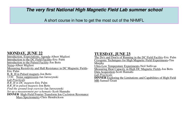
1. The very first National High Magnetic Field Lab summer school A short course in how to get the most out of the NHMFL MONDAY, JUNE 22 Introduction, Expectations, Agenda-Albert Migliori  Introduction to the DC Field Facility-Eric Palm Introduction to the Pulsed Facility-Jon Betts Noise-Albert Migliori Measuring Resistivity and Hall Resistance in DC Magnetic Fields-Eric Palm R, R_H in Pulsed magnets-Jon Betts1330 Noise suppression-Jan Jaroszynski Lab Practicals R,R_H in DC magnets-Eric Palm R,R_H in pulsed magnets-Jon Betts Find the ground loop exercise-Jan Jaroszynski Set up a measurement per schematic-Scott Hannahs DINNER High-Field Fourier Transform Ion Cyclotron Resonance Mass Spectrometry-Chris Hendrickson TUESDAY, JUNE 23The Do's and Don'ts of Running in the DC Field Facility-Eric Palm Cryogenic Techniques for High Magnetic Field Experiments-Tim Murphy Ultra-Low Temperature Experiments-Neil Sullivan Measuring Heat Capacity in High DC Magnetic Fields-Jon Betts Data Acquisition-Scott Hannahs Lab Practicals DINNER Exploring the Limitations and Capabilities of High Field MR-Samuel Grant

2. WEDNESDAY, JUNE 24The Versatility of Magnetic Fields in Condensed Matter Physics, Chemistry and Biology-Greg Boebinger Fermi surfaces in Extreme Magnetic Fields-Neil Harrison Magnetometry at the NHMFL: A Practical Guide to AC Susceptometer, Torque Magnetometer,VSM Users-Eun Sang Choi 1300 FREE TIME DINNEROptical Microscopy for the Material Sciences-Michael Davidson THURSDAY, JUNE 25Infrared and THz spectroscopy at High Magnetic Fields-Dmitry Smirnov The TDO and Beyond: Contactless Methods for High Precision Measurements of Electrical Resistivity-Ross McDonald The Vector Potential and Other Exotica in High Field and Low Temperature Experiments-Jim Brooks Applications of Electron Magnetic Resonance at the NHMFL-Stephen Hill A “Big Light” Terahertz-to-Infrared Laser: Condensed Matter Physics, Chemistry and Biology in the Notorious 'Terahertz Gap-Greg Boebinger NMR for Chemistry and Biology-ZhehongGan Lab Practicals Acquire a spectrum on FTIR, as function of B–Dmitry Smirnov Acquire a spectrum on EMR, as function of B-Steve Hill Cantilevers, cavities-Ross McDonald Acquire a spectrum using NMR-ZhehongGan DINNER NMR for Chemistry and Biology -ZhehongGan FRIDAY, JUNE 26 Ultrafast User Spectroscopy at the NHMFL-Steve McGill Ultrasound (Pulsed and RUS)-Albert Migliori High Pressure Methods for Extreme Condition Research-Stan Tozer Dilatometry-Vivien Zapf Petroleum Analysis by Fourier Transform Ion Cyclotron Resonance Mass Spectrometry-Ryan Rodgers Lab Practicals DINNERSuperconductors for Superconducting Magnets-David Larbalestier SATURDAY, JUNE 27 Student presentations --Each student brings 12 minute talk on pre-assigned paper. Assignments made from list of high-magnetic field papers. Each student presents to fellow students.

3. Noise 101Ohms law (MKS units only please)

4. AC versions

5. Noise and interference How can we hear anything at all on the radio as we drive to work in the morning. The air is filled with transmissions from all the AM and FM radio stations, cellular phones (yuch!), TV, air traffic control, police, fire, medical, business band, ham radio, satellites, radar, model airplanes, cordless phones, garage door openers, GPS, microwave relay links, and much more. In addition, lightning, the ionosphere, power lines, auto ignition, and sunspots all fight to produce interference, while the cosmic background, the thermal radiation from the sun, and from all bodies not at zero (absolute) temperature, produce electromagnetic noise. Any electrical measurement we might like to make is, therefore, made in the presence of four unwanted sources of electrical energy: 1. coherent narrow bandwidth transmissions 2. broadband interference 3. Low-frequency (1/f) fluctuation noise and shot noise 4. true thermal noise sources

6. Types of noise: Coherent narrow-band transmissions are characterized by continuous energy output concentrated in a very narrow band of frequencies at energy densities far above that produced by any thermal noise source we are likely to encounter. Interference sources are contain many frequency components and may be detected by our measurements. 1/f, or fluctuation noise, is very mysterious, and we won’t go into it much. Shot noise occurs when currents (of any sort) are so low that things pop through one at a time. Its effects are statistical and intrinsic. Thermal noise sources (Johnson noise) are characterized by a completely and perfectly incoherent energy output with bandwidth and amplitude exactly determined by temperature.

7. What we are trying to do! Thermal energy produced over a broad range of frequencies is a property of the universe. This not only cannot be blocked, it is produced inside our measuring system. The thermal energy from our own electronics creates electrical noise that we can never eliminate without cooling, a practice widely used by those unconcerned with cost (military, and, in times past, scientists).

8. So, we shield against interference (ignition noise, for example), and the rest is done by making a measurement system that filters out all other unwanted frequencies. • The energy density of the data stream must be greater than the thermal energy present. The reason this is so easy to do well is that the thermal energy is always of specific amplitude at each frequency. More precisely, thermal noise has a relatively constant energy density per unit bandwidth in the frequency range we are interested in. If we can reduce the band of frequencies accepted by our electronics, we can reduce the total thermal noise energy getting in as well.

9. Johnson noise and the fluctuation-dissipation theoremTake 8 coins and throw them on the table, one at a time. There are 256 possible combinations. Here’s how they are distributed. This function rapidly becomes sharp at the 1023 level.

10. Statistical mechanicsThe number of possible states increases rapidly with energy The energy levels are hfapart- discrete energies make it easy to count-so the quantum system is easier to deal with for thermodynamic problems. • With 2 quanta--states are • 200 020 002 110 101 011 • for a total of 6 states. • With 3 quanta--states are • 300 030 003 210 201 120 102 012 021 111 • for a total of 10 states. • If there are 1021 oscillators, then a 10% increase in energy gives about (1.1)^1021=2^1019 more states.

11. Stat Mech continued-Temperature, Entropy, Fluctuations • W(E) is the number of states the system can have with energyE=E1+E2. • Every state is equally likely • W1(E1) states • Energy E1 • W2(E2) states • Energy E2 • What is the probability that we observe this? • This is a very sharply peaked function that is the product of a rapidly increasing function of E1 and a rapidly decreasing one.

12. Temperature and Entropy After a while, no matter what the initial states were, the system is observed near its most likely configurations. Those configurations divide the energy between the two subsystems in a very special way so that the fractional increase in the number of configurations of the smaller system is exactly matched by the fractional decrease in the number of configurations of the large system. This expresses one property common to both systems once things have settled down (reached thermal equilibrium), something we already know about. What we know is that after a while, the temperature of both systems is the same. The definition of the temperature is: We define entropy to be

13. Thermal equilibrium occurs when the temperatures of the subsystems are the same, which is equivalent to saying that the system is very near a maximum probable configuration.What else must be true?(PE is the probability)But this is just the Boltzmann factor that tells us the relative probability of states with different energies!

14. There is a strange property relating to entropy. • If we observe a very probable configuration in the past, we continue to observe a very probable configuration! • But if we arrange the system in a very improbable configuration in the past, it rapidly adjusts itself to a probable one. • Think of a glass of water with one drop of ink in it carefully placed so it just floats there, and another glass with the same amount of ink thoroughly mixed. • Let the glass with the visible drop sit for a day. • Look at both glasses, measure them with everything you’ve got, you cannot tell the difference. • Reverse time for a day. In one glass the drop reappears, in the other, absolutely nothing happens! • Entropy gives us the real arrow of time.

15. The fluctuation-dissipation theorem • Electronic scattering “resets” the distribution of perturbed electrons to a thermal one-that is, one that is more probable. An unrecoverable loss of electrical energy becomes heat. A thermal “force” is responsible so that the randomizing forces (voltages) generate : • fluctuations (noise) and • b) a slowly varying time averaged force that depends on the velocity (resistance) such that any undriven current started in a resistor must decay to zero after a while. • let’s see how!

16. The process In a resistor with a static applied electric field E, each electron sees Where ET(t) are the random thermal forces associated with scattering. All we need to show is that a reasonable time average of this produces a velocity-dependent force. Then, just what is needed to dissipate currents.

17. Averages • We are going to compute averages. We can either average over lots of different resistors, or over one resistor at lots of different times–these are equivalent. • If we know the velocity of the charge at time t, what is it a little later at t+Dt ? • This is the process where we average over different times in the same resistor, rather than over many resistors at one time. • Dt is very short compared to the time over which E varies, but very long compared to electronic scattering times (10-14s), so we get a good take on the average of the fluctuations.

18. Now ET(t) is wildly varying, and in thermal equilibrium has an average of zero, but not so out of equilibrium. We now replace the instantaneous field with its average over long times (which is not zero) so that: • We also know that thermal energyDQiis being added to the bath at the expense of electrical energy from the source in some unknown way. • As the bath heats, the number of its configurations goes up. So does the probability P1of any configuration near the small region associated with the charge we are studying, ie. so that • ifDQiis small

19. Let’s now track this same state as the bath heats. We can compute its value of electric field by summing over all states weighted by changed probabilities. remember that at equilibrium, there is no average force, so we lose one term. This is the spot where things really happen! lets conserve energy (always nice)! Work=force x distance Combine to get a velocity-dependent electric field that is just what is needed to relax the electric current. remember, v(t) is varying very slowly

20. But we know that is the electric field developed after a very short time (a few scattering times). That’s our field! • We also define resistivity by E=r Je, ( , n is the number of charges/unit volume) so that: the electrical resistivity is then: where we knew the integrand went to zero fast , so we could change the limits to +/- infinity and divide by 2 to correct. This is the fluctuation-dissipation theorem, with velocity dependent force (viscous drag). Note that resistivity is now tied to important microscopic and thermodynamic stuff, and in fact depends on the E-field/E-field correlation function, which is what is in the integral. We will now pick at this, but first....

21. Correlation Functions • is the E-field/E-field correlation function. • It tells us how well we know the electric field at t+Dt if we know it at t. • It contains NO fluctuations, it only tells about the smooth average processes. • For the resistor, it is required that after scattering occurs, directions are random so that: • averages to zero for Dt greater than l/vf and is equal to E2 for times less than this. • Thus scattering acts as a near delta function. Its Fourier transform has frequency components up to the scattering rate, and little above this.

22. The correlation limit • Now, where at • times shorter than the scattering rate, determined by Dt0=vf/l=2p/Dw0, • ET(t)=ET(t+t’). The Fourier transform of this spike gives Johnson noise. • For frequencies less than the scattering rate (1014 Hz in a metal at room temperature), the RMS noise electric field is • Remember, this is the electric field noise with bandwidth in units of angular frequency (2pf). To get voltages, we need to construct a resistor and compute the voltage noise.

23. Resistors • If we make a resistor out of this material (go from fields to voltages), • using frequency (not angular frequency). • where has units volts squared. • Also • Note that real resistors suffer other fluctuations such that excess noise is generated. • This noise is 1/f like and is sort-of constant per decade of bandwidth. • The levels per decade are about 0.1mV to 3.0mV for carbon resistors, 0.05mV to 0.3mV for carbon film, and less than 0.02mV for good metal film.

24. Shot Noise: The other naturally required noise component • Shot noise is caused by the simple statistical fluctuations that occur when charge is carried by quantized units (mostly electrons) and they are uncorrelated. Charge transport in semiconductors is generally uncorrelated, but metallic conduction is not because the electron eigenstates extend over the entire metallic volume and are very correlated. • The shot noise is • where D f is the bandwidth over which measurement is made. • For I=1 amp, Inoise=57nA/(Hz)1/2, etc.

25. A weird limit • Note that the thermal noise voltage is • and the shot voltage noise is • so that when the voltage across the resistor exceeds • =50mV at room temperature, then the noise is dominated by shot noise!! • The shot noise amplitude has also been used to determine the charge magnitude in Quantum Hall Effect systems!! • ----end of noise!

26. The very strongest thermodynamic arguments relate: • fluctuations (noise) to • dissipation (resistance) • making “Johnson noise” • Johnson noise is “white” (up to the correlation limit vf / l=1014 Hz in a metal at room temp). The current noise is In=Vn /R. • A 100W resistor has a noise voltage density of 1.27nV/Hz1/2 at room temperature. For a bandwidth of 100kHz this is about 0.4mV RMS. • Counting statistics are the cause of “shot noise”= • If the voltage across the resistor exceeds = 50mV at room temperature, the noise is dominated by shot noise. But only in systems in which the carriers are statistically independent. This does NOT include good metals.