Download
1 / 38
380 likes | 485 Vues
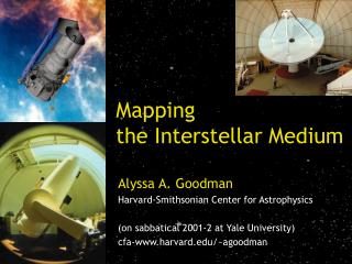
Observational Magnetohydrodynamics of the Interstellar Medium. Alyssa A. Goodman Harvard-Smithsonian Center for Astrophysics. Principal Collaborators Héctor Arce , CfA Javier Ballesteros-Paredes, AMNH Sungeun Kim, CfA Paolo Padoan , CfA Erik Rosolowsky , UC Berkeley

E N D
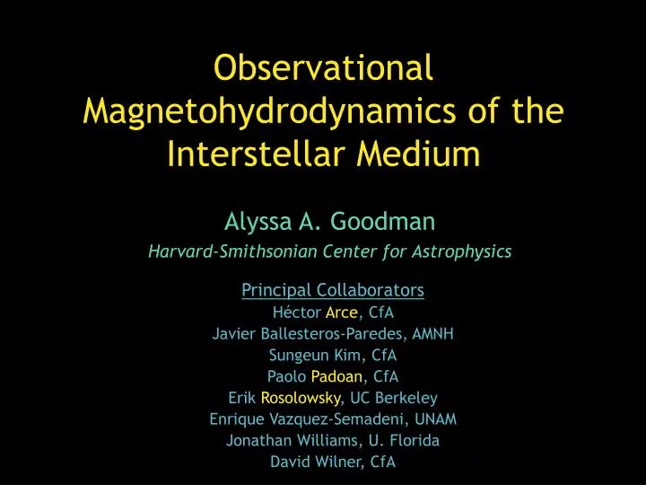
Observational Magnetohydrodynamics of the Interstellar Medium Alyssa A. Goodman Harvard-Smithsonian Center for Astrophysics Principal Collaborators Héctor Arce, CfA Javier Ballesteros-Paredes, AMNH Sungeun Kim, CfA Paolo Padoan, CfA Erik Rosolowsky, UC Berkeley Enrique Vazquez-Semadeni, UNAM Jonathan Williams, U. Florida David Wilner, CfA
Observational MHD of the ISM The Good Old Days • Low Resolution, Observationally & Computationally Spherical, Smooth, Long-lasting “Cloud” Structures And “structure” came from fragmentation
Observational MHD of the ISM The “New Age” • High(er) Resolution, Observationally & Computationally Highly irregular structures, many of which are “transient” on long time scales
“Observational” MHD of the ISM The “New Age” • High(er) Resolution, Observationally & Computationally Highly irregular structures, many of which are “transient” on long time scales Stone, Gammie & Ostriker 1999 Stone, Gammie & Ostriker 1999 And “structure” comes from turbulence on all but smallest scales
What can we actually observe?Intensity(position, position,velocity) Falgarone et al. 1994
Velocity is the Observer’s "Fourth" Dimension Loss of 1 dimension No loss of information
1950 1960 1970 1980 1990 2000 8 10 4 10 7 10 N 6 channels, 10 channels 3 10 *N N 5 10 channels pixels S/N in 1 hour, 2 10 4 10 (S/N)*N N 3 10 1 N 10 pixels pixels 2 10 0 10 1950 1960 1970 1980 1990 2000 Year How Many Bits? Product S/N
Most previous attempts discard or compress either position or velocity information Statistical Tools • Can no longer examine “large” spectral-line maps or simulations “by-eye” • Need powerful, discriminatory tools to quantify and intercompare data sets • Previous attempts are numerous: ACF, Structure Functions, Structure Trees, Clumpfinding, Wavelets, PCA, D-variance, Line parameter histograms
1997 Goals of the “Spectral Correlation Function” Project • Develop “sharp tool” for statistical analysis of ISM, using as much data of a data cube as possible • Compare information from this tool with other statistical tools applied to same cubes • Incorporate continuum information • Use best suite of tools to compare “real” & “simulated” ISM • Adjust simulations to match, understanding physical inputs • Develop a (better) prescription for finding star-forming gas
[ ] T / 10 K b = [ ] 2 -3 [ ] n B m / 100 cm / 1 . 4 G H 2 Strong vs. Weak B-Field b=0.01 b=1 • DrivenTurbulence; M K; no gravity • Colors: log density • Computational volume: 2563 • Dark blue lines: B-field • Red : isosurface of passive contaminant after saturation Stone, Gammie & Ostriker 1999
The Spectral Correlation Function • v.1.0 Simply measures similarity of neighboring spectra(Rosolowsky, Goodman, Wilner & Williams 1999) • S/N equalized, observational/theoretical comparisons show discriminatory power • v.2.0 Measures spectral similarity as a function of spatial scale(Padoan, Rosolowsky & Goodman 2001) • Noise normalization technique found • SCF(lag) even more powerful discriminant • Applications • Finding the scale-height of face-on galaxies!(Padoan, Kim & Goodman 2001) • Understanding behavior of atomic ISM(e.g. Ballesteros-Paredes, Vazquez-Semadeni & Goodman 2001)
Measures similarity of neighboring spectra within a specified “beam” size lag & scaling adjustable signal-to-noise accounted for How SCF v.1.0 Works See: Rosolowsky, Goodman, Wilner & Williams 1999; Ballesteros-Paredes, Vazquez-Semadeni & Goodman 2001
Antenna Temperature Map Application of the “Raw” SCF greyscale: TA=0.04 to 0. 3 K “Raw” SCF Map Data shown: C18O map of Rosette, courtesy M. Heyer et al. Results: Padoan, Rosolowsky & Goodman 2001 greyscale: while=low correlation; black=high
greyscale: TA=0.04 to 0. 3 K Antenna Temperature Map Application of the SCF “Normalized” SCF Map Data shown: C18O map of Rosette, courtesy M. Heyer et al. Results:Padoan, Rosolowsky & Goodman 2001. greyscale: while=low correlation; black=high
Normalized C18O Data for Rosette Molecular Cloud Randomized Positions Original Data SCF Distributions
Unbound High-Latitude Cloud Self-Gravitating, Star-Forming Region Observations Simulations No gravity, No B field No gravity,Yes B field Yes gravity, Yes B field Insights from SCF v.1.0Rosolowsky, Goodman, Williams & Wilner 1999
1.0 0.8 0.6 Rosette C 18O Rosette 13CO Increasing Similarity of ALL Spectra in Map Rosette 13CO Peaks SNR 0.4 HCl2 C 18O H I Survey L134A 13CO(1-0) Rosette C 18O Peaks Pol. 13CO(1-0) L1512 12CO(2-1) 0.2 HCl2 C 18O Peaks L134A 12CO(2-1). HLC 0.0 0.0 0.2 0.4 0.6 0.8 1.0 1.2 Which of these is not like the others? Increasing Similarity of Spectra to Neighbors Change in Mean SCF with Randomization G,O,S MacLow et al. Falgarone et al. Mean SCF Value
v.2.0: Scale-Dependence of the SCF Example for “Simulated Data” Padoan, Rosolowsky & Goodman 2001
“A Robust Statistic” Padoan, Rosolowsky & Goodman 2001
Galactic Scale Heights from the SCF (v.2.0) HI map of the LMC from ATCA & Parkes Multi-Beam, courtesy Stavely-Smith, Kim, et al. Padoan, Kim & Goodman 2001
Insights into Atomic ISM from SCF (v.1.0) Comparison with simulations of Vazquez-Semadeni & collaborators shows: • “Thermal Broadening” of H I Line Profiles can hide much of the true velocity structure • SCF v.1.0 good at picking out shock-like structure in H I maps (also gives low correlation tail) See Ballesteros-Paredes, Vazquez-Semadeni & Goodman 2001.
How is the MHD turbulence driven in the dense ISM? pc-scale outflows?
“Giant” Herbig-Haro Flows:PV Ceph 1 pc Reipurth, Bally & Devine 1997
67:55 H H 3 1 5 C 1 5 B H H 3 H H 3 1 5 A 67:50 H H 4 1 5 HH 215P2 ) 0 HH 215P1 5 9 1 PV Cephei ( d 67:45 HH 315D H H 3 1 5 E 67:40 H H 3 1 5 F 20:46 20:45 ( 1 9 5 0 ) a Giant HH Flow in PV Ceph 12CO (2-1) OTF Map from NRAO 12-m Red: 3.0 to 6.9 km s-1 Blue: -3.5 to 0.4 km s-1 Arce & Goodman 2001
Driving Turbulence with Outflows Studies in Héctor Arce’s Ph.D. Thesis (Harvard, 2001; see Arce & Goodman 2001 a,b,c,d) show: • HH 300 outflow has ~enough power(~0.5 Lsun at a 1-pc scale) to drive turbulence in its region of Taurus (using estimates based on Gammie & Ostriker 1996) • Many outflows show clear evidence for “episodicity” and this may effect coupling of outflow energy to cloud • Episodicity may also explain steep mass-velocity relations, and odd-looking p-v diagrams • Outflow sources move through the ISM (e.g. PV-Ceph)
NGC 2264G g~1.8 g~3.5 Lada, C.J. & Fich, M. 1996, ApJ,.459, 638
FIG. 10.Northeast lobe of the IRS 1 flow. (a) Area-integrated spectrum of region R2 in 12CO J = 2 1 (solid line), 12CO J = 10 (dotted line), and 13CO J = 10 (dashed line). (b) Fit to the ratio of optical depths R12/13 = (12CO J = 10)/(13CO J = 10), integrated over the region. Valid points kept for the fit are those with ratios with both intensities above twice the rms noise and for velocities outside the turbulent line core (diamonds). Invalid points not meeting those criteria are indicated by a cross. The second-order polynomial fit to the valid points is shown as a solid curve. The dashed line is the result of fitting a parabola to the entire cloud in region R1. Vertical dashed lines outline the turbulent line core (cloud vLSR ± 0.75 km s-1). (c) Luminosity mass vs. inclination-corrected velocity from center of the flow. Lines show fits to the power law ML v-. Points for the blueshifted lobe are indicated by diamonds; the redshifted lobe points by triangles. Filled symbols denote masses calculated directly from 13CO J = 10; open symbols denote masses calculated from the fit of the optical depth ratio. (d, e, and f) Same as (a), (b), and (c) except that they are for the southwest lobe of the IRS 1 flow (region R3). B5 FIG. 11.Northeast lobe of the IRS 1 flow with the ambient cloud subtracted out. (a) Area-integrated 12CO J = 21 emission in region R2 (thin line); same emission with the ambient cloud (defined by region R4) subtracted out (thick line). (b and c) Same as for Fig. 10. (d, e, and f) Same as (a), (b), and (c) except that they are for the southwest lobe of the IRS 1 flow (region R3 in Fig. 9) with the ambient cloud (region R5 in Fig. 9) subtracted out. Yu, Billawala, Bally, 1999
L1448 Bachiller, Tafalla & Cernicharo 1994 Lada & Fich 1996 B5 Yu Billawala & Bally 1999 Bachiller et al. 1990 Sample outflow position-velocity diagrams
Outflow position-velocity diagrams Arce & Goodman 2001
Variations in Burst History… e.g. NGC2264 Single or Dominant “Hubble” Flow e.g. L1448 Sorted “Hubble” Wedges Velocity e.g. B5, HH300 Random “Hubble” Wedges Position
A,B,C... for constant vmax a,b,c... for varying vmax (alphabetical=chronological) a 1 2 d A C B 3 D E 4 6 5 7 c e 8 b Mass-Velocity & Position-Velocity Relations in Episodic Outflows 0 10 10 Power-law Slope of Sum = -2.7 Slope of Each Outburst = -2 -1 10 8 -2 10 6 Mass [Msun] Maximum Velocity, vmax -3 10 4 -4 10 -5 10 2 2 3 4 5 6 7 8 2 3 4 5 6 7 8 2 2 4 6 8 10 0.1 1 10 Velocity [km s-1] Maximum Offset from Source, dmax Arce & Goodman 2001
Time-Ordering of p-v Diagrams? a d e c b a d e c b a d e c b
Episodic ejections from precessing or wobbling moving source PV Ceph Required motion of 0.25 pc (e.g. 2 km s-1 for 125,000 yr or 10 km s-1 for 25,000 yr) Arce & Goodman 2001
Even leaves a trail? Arce & Goodman 2001
Outflows Driving Turbulence • What you see (now) is not the whole story. • Outflows seem to have a complex time-history. • Sources may travel. • Questions Raised: • Is true net momentum/energy input is still measurable from observations? • Do simulations need to include time history, or is “net” enough? • How do we find all the flows?