Download
1 / 9
90 likes | 216 Vues
LES of Turbulent Flows : Lecture 9 (ME EN 7960-003). Prof. Rob Stoll Department of Mechanical Engineering University of Utah Fall 2014. Subgrid -Scale Modeling.

E N D
LES of Turbulent Flows: Lecture 9(ME EN 7960-003) Prof. Rob Stoll Department of Mechanical Engineering University of Utah Fall 2014
Subgrid-Scale Modeling • One of the major hurdles to making LES a reliable tool for engineering and environmental applications is the formulation of SGS models and the specification of model coefficients. • Recall: we can define 3 different “scale regions” • in LES depicted in the figure to the right => Resolved Scales, Resolved SFS, SGSs • We can also decompose a general variable as: • When we talk about SGS models we are specifically talking about the scales below ΔNOT the Resolved SFS. Resolved SFS π/Δ π/Δ SGSs Resolved scales
Modeling τij • see Pope pgs. 582-583 or Sagaut pgs. 49-50, 59-60 (this will mostly follow Sagaut) • we can decompose the nonlinear term as follows (using ): • we now have the nonlinear term as a function of and . • two different basic forms of the decomposition (based on the above equation are prevalent) • The 1st one is based on the idea that all terms appearing in the evolution of a filtered quantity should be filtered: • where • and
Modeling τij (continued) • -A 2nd definition can be obtained by further decomposition of => • Lij => Leonard stress (the interaction among • the smallest resolved scales) • Our total decomposition is now: • (Leonard, Adv. in Geo., 1974) • If our filter is a Reynolds operator (e.g., cutoff filter) Cij and Lij vanish! • NOTE: while τij is invariant to Galilean transformations, Lij and Cijare NOT. Because of this, the decomposition given above (for the most part) is not used anymore (although we will see similar terms again in our SGS models) • A more rigorous decomposition was proposed by Germano into generalized filtered moments. Under this framework the generalized moments look just like “Reynolds” moments, our original τij! (see Germano, JFM, 1992 in the handouts section. This is also recommended reading for a discussion of filtering and the relationship between LES filters and Reynolds operators)
Classes of LES Models (for τij) • Eddy-Viscosity Models: • The largest and most commonly used class of SGS models • The general idea is that turbulent diffusion at SGSs (i.e. how SGS remove energy) is analogous to molecular diffusion. It is very similar in form to K-theory for Reynolds stresses. • The deviatoric part of τij is modeled as: • where νT is the SGS eddy-viscosity and • Within this class of models we have many different ways of determining νT • Smagorinsky model (Smagorinsky, Mon. Weath. Rev., 1963) • “Kolmolgorov” eddy-viscosity (Wong and Lilly, Phys. of Fluids, 1994) • Two-point closure models (based on Kraichan’s (JAS, 1974) spectral eddy-viscosity model and developed by Lesiour (see Lesiour et al., 2005) • One-equation models that use the filtered KE equation (see Lecture 6 for the KE equation and Deardorff (BLM, 1980) for an early application of the model)
Classes of LES Models (for τij) • Similarity Models: • Based on the idea that the most active SGS are those close to the cutoff wavenumber (or scale) these models were first introduced by Bardina et al. (AIAA, 1980). A subclass under this type of model is the nonlinear model. Many times these models are paired with an eddy-viscosity model. • Stochastic SGS models: • In these models a random (stochastic) component is incorporated into the SGS model. Usually the nonlinear term is combined with an eddy-viscosity model in a similar manner to the similarity models (Mason and Thomson, JFM, 1992). • Subgrid Velocity Reconstruction Models: • These models seek to approximate the SGS stress through a direct reconstruction of the SGS velocity or scalar fields. Two examples are: • - fractal models (Scotti and Meneveau, Physica D, 1999) • - Linear-eddy and ODT models (Kerstein, Comb. Sci. Tech, 1988) • Dynamic Models: • Actually more of a procedure that can be applied with any base model, first developed by Germano (Phys of Fluids, 1991). • One of the biggest and most influential ideas in LES SGS modeling.
Testing SGS Models • How do we test SGS models? • a posteriori testing (term can be credited to Piomelli et al., Phys of Fluids, 1988) • Run “full” simulations with a particular SGS model and compare the results (statistically) to DNS, experiments and turbulence theory. • A “complete” test of the model (including dynamics and feedback) but is has the disadvantage of including numerics and we can’t gain insight into the physics of SGSs. • a priori testing (term can be credited to Piomelli et al., Phys of Fluids, 1988) • Use DNS or high resolution experimental data to test SGS models “offline” • Goal: directly compare with by: • Filter DNS (or experimental) data at Δ and compute the exact and other relevant parameters (e.g., Π) • Use the filtered u,v and w to compute from the model (and stats) and compare with above results (this can also be used to calculate unknown model coefficients) • Allows us to look specifically at how the model reproduces SGS properties and the physics associated with those properties • Drawback, it doesn’t include dynamic feedback and numerics!
Eddy viscosity Models • Eddy Viscosity Models: (Guerts pg 225; Pope pg 587) • Above, we noted that eddy-viscosity models are of the form: • momentum: • scalars: • -This is the LES equivalent to 1st order RANS closure (k-theory or gradient transport theory) and is an analogy to molecular viscosity (see Pope Ch. 10 for a review) • -Turbulent fluxes are assumed to be proportional to the local velocity or scalar gradients • -In LES this is the assumption that stress is proportional to strain: • -The SGS eddy-viscosity must still be parameterized. filtered strain rate eddy-viscosity SGS Prandtl number eddy-diffusivity
Eddy viscosity Models • Dimensionally => • In almost all SGS eddy-viscosity models • Different models use different and • Recall the filtered N-S equations: • Note, for an eddy-viscosity model we can write the viscous and SGS stress terms as: • We can combine these two and come up with a new (approximate) viscous term: • What does the model do? We can see it effectively lowers the Reynolds number of the flow and for high Re (when 1/Re=>0), it provides all of the energy dissipation. length scale velocity scale