Download
1 / 26
270 likes | 507 Vues
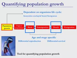
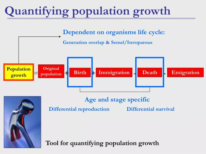
Original population. Population growth. =. +. +. Immigration. -. Death. -. Emigration. Birth. Tool for quantifying population growth. Quantifying population growth. Dependent on organisms life cycle: Generation overlap & Semel/Iteroparous. Age and stage specific.

E N D
Original population Population growth = + + Immigration - Death - Emigration Birth Tool for quantifying population growth Quantifying population growth Dependent on organisms life cycle: Generation overlap & Semel/Iteroparous Age and stage specific Differential reproduction Differential survival
Life tables Raw count data Raw count data Reproductive output Life history features Converse = survival rate px = 1 - qx
R0 is the population’s replacement rate: If R0 = 1.0…no population growth If R0 < 1.0…the population is declining If R0 > 1.0…the population is increasing Non-overlapping generations Makes explicit the dependence of r on the reproduction of individuals (R0) and the length of generation (Tc) Overlapping generations Population characteristics • R0 =the basic reproductive rate • Tc = cohort generation time • ex = life expectancy • r = intrinsic growth rate Can use life tables to determine characteristics about the population:
Constant survival rates Constant rates of reproduction Rarely the case! Stable age structure lx r = intrinsic rate of natural increase that the population has the potential to achieve. time More on r (the intrinsic growth rate) BUT still useful to characterise a population in terms of its potential…especially when trying to make comparisons e.g. between populations of the same species in different environments to see which environment is more favourable for the species. Stable r
Non-overlapping generations Overlapping generations Life tables – merits and shortcomings Life tables useful – particularly for organisms with simple life histories Life tables less informative for organisms with complex life histories Population growth potential POPULATION PROJECTION More general and useful method of analysing and interpreting the survival and fecundity schedules of population with overlapping generations
Projecting population change Projecting doesn’t forecast what WILL happen Projects forward to what WOULD happen if fecundity and survival schedulesremained the same over time Key pieces of information are for projecting: p = survival rate m = fecundity (individuals produced per surviving individual) Certain steps must be followed to project data…
Projecting population change 1. Rearrange data(Copy < Paste Special < Transpose)
* * * = = = Projecting population change 2. Calculate survivorship for x1 to xn Make sure that references to the p-values are absolute ($ signs) and that references to the X-values are relative (no $ signs) Based on the px values (survival rate) we can calculate the size of each age class at t+1 based on the size of the age class at time t X1=Xt*px Copy formula down
* * * Projecting population change Make sure that references to the m-values are absolute ($ signs) and that references to the X-values are relative (no $ signs) 3. Add fecundity to x0 column Based on the mx values (fecundity) we can calculate the number of new individuals produced per individual at each age Based on the mx values (fecundity rate) we can calculate the number of individuals produced for each individual in each age class X0 = X1*mx + X1*mx+ X1*mx Copy formula down
=sum(all x-values) Projecting population change 4. Calculate R (fundamental reproductive rate) • Calculate Nt (size of each generation) • Calculate R (fundamental reproductive rate) Copy ALL formulas down until R stabilises….
Eventually R stabilises….in this case it did so after ≈ 72 generations
Nt R NOTE: when R stabilises, so too does the age-structure, and this is known as the stable-age distribution of the population. The proportions of the stable-age distribution are termed Cx To calculate Cx: - Where R is stable, calculate the proportions of each age class in the generation Cx
Projecting population change With a constant r (lnR) and a constant stable age distribution (Cx)we can now calculate the fecundity and survival rates of the population… Constant survival rates Constant rates of reproduction r (lnR) Stable r Stable age structure time lx
Birth rate (B) = number of births/number of reproducing individuals Survival rate (S) = No Survivors at time t, divided by total population size at time t-1 Projecting population change Nt+1 = Nt.(Survival Rate) + Nt.(Survival Rate).(Birth Rate) So, at stable-age distribution: B = 8.77 S = 0.24 Rearrange Nt+1 = Nt.(Survival Rate).(1 + Birth Rate) Must calculate Birth Rate and Survival Rate
All life history components affect this contribution – ultimately through fecundity and survival But necessary to combine these effects into single currency so that different life history strategies may be judged Reproductive value (RVx) Individual contributions Natural selection favours those individuals that make the greatest proportionate contribution to the future of the population to which they belong Consider the contribution of each individual…
CURRENT reproductive output (mx) FUTURE reproductive output (Vx*) vx* = residual reproductive value CURRENT reproductive output (mx) FUTURE reproductive output (Vx*) Reproductive value • Sum of the current reproductive output (mx) and the future (residual) reproductive value (Vx*) • Vx* combines expected future survival and expected future fecundity • This is done in a way that takes account of the relative contributions of individual to future generations • The life history favoured by natural selection is the one for which the sum of contemporary output and Vx* is the highest vx = mx + vx*
15 Time of greatest contribution to future generations 10 Reproductive value Data for an annual plant 5 0 Age (days) 50 100 150 200 250 300 350 400 8 6 Reproductive value 4 Time of greatest contribution to future generations 2 Data for a sparrowhawk 0 0 2 4 6 8 10 Age (years) Reproductive value
This expression can ONLY be used to calculate vx* IF the time intervals used in the life table are equal. vx* = [(vx+1.lx+1) / (lx.R)] * ∑ * Copy formula up Copy formula up Reproductive value To calculate Vx vx = mx + vx* To calculate vx* work backwards in the life-table, because vx* = 0 in the last year of life
Age where contribution of an individual to future generations is greatest relative to the contribution of others in the population Reproductive value Reproductive value Age
Original population Population growth = + + Immigration - Death - Emigration Birth So far… Dependent on organisms life cycle: Generation overlap & Semel/Iteroparous Age and stage specific Differential reproduction Differential survival Birth Pulse Birth Flow
Single Leaving Event Reproduction Reproduction 30 Constant Addition and Leaving mx 20 mx 10 0 0 1 2 Age class Age class Birth flow vs. Birth pulse BIRTH Projecting with birth flow Pulse Flow • constant addition and leaving of individuals • reproduction is spread across an age class
mx-1 mx Birth flow vs. Birth pulse Dealing with Birth FLOW: Need to adjust mx values to reflect FLOW rather than PULSE. Then project data as normal with new mx values. • Assume that all reproduction occurs at the mid-point of an age-class. • The mx values are appropriate for the end of an x class - not at the middle - need get average….To get at average of mx and mx+1 = (mx-1 + mx)/2 mx Age
Need to consider survival from period x-1 through x to x+1: i.e. px = [(lx + lx+1)] / [(lx + lx-1)] Calculate a new px value mx* = ((mx-1 + pxmx)/2 Use formula to adjust mx with new px value Birth flow vs. Birth pulse This is the basic life table (birth pulse) that we have constructed so far: Projections are based on mx MUST ADJUST mx HOW?
* Birth flow vs. Birth pulse NOTE: px values used in the life tables, and calculations therein, do not change. i.e. px (birth-flow) = px (birth-pulse) and the revised px values above are only used to calculate mx values. Need to consider survival from period x-1 through x to x+1: i.e. px = [(lx + lx+1)] / [(lx + lx-1)] 1. Calculate a new px value mx* = ((mx-1 + pxmx)/2 2. Use formula to adjust mx with new px value 3. Change formulas for x0 to use mx* instead of mx 4. Copy new formula down until R stabilises
Birth flow vs. Birth pulse BIRTH PULSE BIRTH FLOW R stabilised after 72 generations at 5.07 Both populations are growing (R>1) but the birth pulse population is growing more quickly R=1.26 vs R=5.07 R stabilised after 41 generations at 1.26
Projecting population change Steps of projecting data: • Rearrange data from rows to columns • Calculate projected survivorship for x1 to xn • Calculate projected fecundity for x1 to xn • For each x calculate Nt and Nt+1 • For each x calculate R (Nt+1/Nt) • Copy the formulas down until R stabilises • Calculate the proportions of each class where R is stable (ax /Nt) to calculate stable age class distribution (cx)