Download
1 / 22
220 likes | 355 Vues
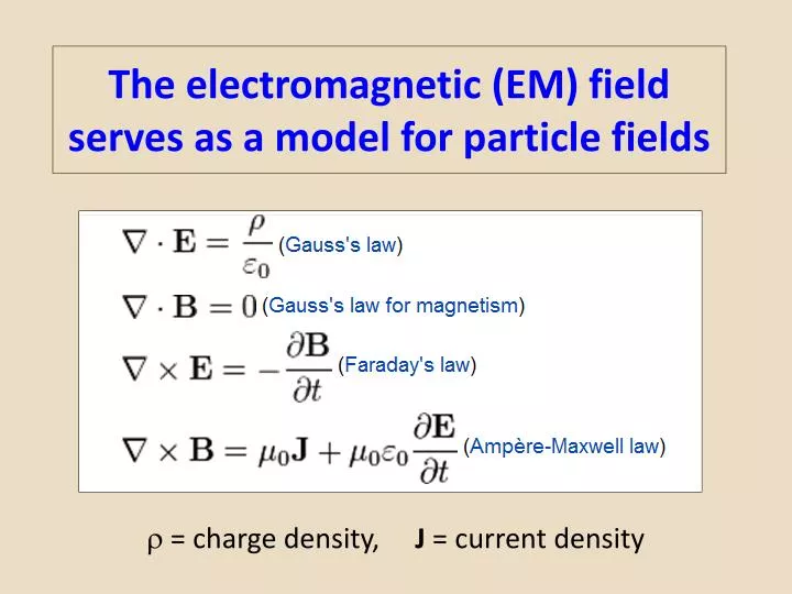
The electromagnetic (EM) field serves as a model for particle fields. = charge density, J = current density. 4-vector representation of EM field. A is the vector potential is the electrostatic potential ; c = speed of light. How E and B are related to . Derivation of E.

E N D
The electromagnetic (EM) fieldserves as a model for particle fields = charge density, J = current density
4-vector representation of EM field • A is the vector potential • is the electrostatic potential; • c = speed of light
How E and B are related to Derivation of E
Wave equations for A and Lorentz gauge! = 0
The µ µ operator Summation implied!
The wave equations for A and can be put into 4-vector form:
The sources: charges and currents The sources represent charged particles (electrons, say) and moving charges . They describe how charges affect the EM field!
represents four 4-dim partial differential equations – in space and time!
If there are no electrons or moving charges: This is a “free” field equation – nothing but photons! We will look at solutions to these equations.
Solutions to 1. We have seen how Maxwell’s equations can be cast into a single wave equation for the electromagnetic 4-vector, Aµ . This Aµ now represents the E and B of the EM field … and something else: the photon! • If Aµ is to represent a photon – we want it to be able to represent • any photon. That is, we want the most general solution to the equation:
First we assume the following form, We are left with solving the following equation:
creation operator annihilation operator Spin vector Spin vector This “Fourier expansion” of the photon operator is called “second quantization”. Note that the solution to the wave equation consists of a sum over an infinite number of “photon” creation and annihilation terms. Once the ak± are interpreted as operators, the A becomes an operator.
The A is not a “photon”. It is the photon field “operator”, which stands ready to “create” or “annihilate” a photon of any energy, , and momentum, k.
Recall that in order to satisfy the four wave equations the following had to be satisfied. This gives a relativistic four-momentum for a particle with zero rest mass! Note that = |k| c = (m0c)2 “rest” frame
creation & annihilation operators The procedure by which quantum fields are constructed from individual particles was introduced by Dirac, and is (for historical reasons) known as second quantization. Second quantization refers to expressing a field in terms of creation and annihilation operators, which act on single particle states: |0> = vacuum, no particle |p> = one particle with momentum vector p
Notice that for the EM field, we started withthe E and B fields –and showed that the relativistic “field” was a superposition of an infinite number of individual “plane wave” particles, with momentum k . The second quantization fell out naturally. This process was, in a sense, the opposite of creating a field to represent a particle. The field exists everywhere and permits “action at a distance”, without violating special relativity. We are familiar with the E&M field!
In this course we will only use some definitions and operations. These are one particle states. It is understood that p = k. Our definition of a one particle state is |k>. We don’t know where it is. This is consistent with a plane wave state which has (exactly) momentum p: x px /2 The following give real numbers representing the probability of finding one particle systems – or just the vacuum (no particle). vacuum one particle This is a real zero!
Here is a simple exercise: On the other hand,
How might we calculate a physically meaningful • number from all this? • Some things to think about: • The field is everywhere – shouldn’t we integrate over all space? • Then, shouldn’t we make the integration into some kind of • expectation value – as in quantum mechanics? • It has to be real, so maybe we should use A*A or something similar? • How about <k| A*A dV |k> ? • What do you think? • Maybe we should start with a simpler field to work all this out! • The photon field is a nice way to start, but it has spin – and a • few complications we can postpone for now.
One final comment on the electromagnetic field: conservation of charge The total charge flowing out of a closed surface / sec = rate of decrease of charge inside a Lorentz invariant!