Download
1 / 21
240 likes | 644 Vues
Temperature and pressure coupling. MD workshops 26-10-2004. Why control the temperature and pressure?. isothermal and isobaric simulations (NPT) are most relevant to experimental data constant NPT ensemble: constant number of particles, pressure, and temperature.

E N D
Temperature and pressure coupling MD workshops 26-10-2004
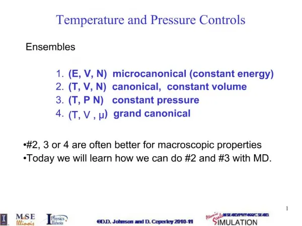
Why control the temperature and pressure? • isothermal and isobaric simulations (NPT) are most relevant to experimental data • constant NPT ensemble: constant number of particles, pressure, and temperature
Causes of temperature and pressure fluctuations the temperature and pressure of a system tends to drift due to several factors: • drift as a result of integration errors • drift during equilibration • heating due to frictional forces • heating due to external forces
Temperature coupling methods in GROMACS weak coupling • exponential relaxation Berendsen temperature coupling (Berendsen, 1984) extended system coupling • oscillatory relaxation Nosé-Hoover temperature coupling (Nosé, 1984; Hoover, 1985)
Berendsen temperature coupling • there is weak coupling to an external ‘heat bath’ • deviation of system from a reference temperature To is corrected • exponential decay of temperature deviation
the temperature of a system is related to its kinetic energy, therefore, the temperature can be easily altered by scaling the velocities vi by a factor λ • is the temperature coupling time constant • need to specify in input file (*.mdp file)
Some notes on Berendsen weak coupling algorithm • very efficient for relaxing a system to the target temperature • prolonged temperature differences of the separate components leads to a phenomenon called ‘hot-solvent, cold-solute’, even though the overall temperature is at the correct value Solutions: • apply temperature coupling separately to the solute and to the solvent problem with unequal distribution of energy between the different components
solutionscontinued … • stochastic collisions (Anderson, 1980) - a random particle’s velocity is reassigned by random selection from the Maxwell-Boltzmann distribution at set intervals does not generate a smooth trajectory, less realistic dynamics • extended system (Nosé, 1984; Hoover 1985) - the thermal reservoir is considered an integral part of the system and it is represented by an additional degree of freedom s - used in GROMACS
Nosé-Hoover extended system • canonical ensemble (NVT) • more gentle than Anderson where particles suddenly gain new random velocities • the Hamiltonian is extended by including a thermal reservoir term s and a friction parameter ξ, in the equations of motion H = K + V + Ks + Vs
Nosé-Hoover extended system • The particles’ equation of motion: • ξ is a dynamic quantity with its own equation of motion: • is proportional to the temperature coupling time constant (specified in *.mdp file)
the strength of coupling between the reservoir and the system is determined by - when is too high slow energy flow between system and reservoir - when is too low rapid temperature fluctuations
Nosé-Hoover produces an oscillatory relaxation, it takes several times longer to relax with Nosé-Hoover coupling than with weak coupling • can use Berendsen weak coupling for equilibration to reach desired target, then switch to Nosé-Hoover • Nosé-Hoover chain: the Nose-Hoover thermostat is coupled to another thermostat or a chain of thermostats and each are allowed to fluctuate
Pressure coupling • The system can be coupled to a ‘pressure bath’ as in temperature coupling weak coupling: exponential relaxation Berendsen pressure coupling extended ensemble coupling: oscillatory relaxation Parrinello-Rahman pressure coupling (Parrinello and Rahman, 1980, 1981, 1982)
Berendsen pressure coupling • equations of motion are modified with a first order relaxation of P towards a reference Po • rescaling the edges and the atomic coordinates ri at each step by a factor u leads to volume change • u is proportional to β which is the isothermal compressibility of the system and which is the pressure coupling time constant. Both values must be specified in *.mdp file
Berendsen scaling can be done: 1. isotropically – scaling factor is equal for all three directions i.e. in water 2. semi-isotropically where the x/y directions are scaled independently from the z direction i.e. lipid bilayer 3. anisotropically – scaling factor is calculated independently for each of the three axes
Parrinello-Rahman pressure coupling • volume and shape are allowed to fluctuate • extra degree of freedom added, similar to Nosé-Hoover temperature coupling, the Hamiltonian is extended box vectors and W-1 are functions of M • W-1determines the strength of coupling have to provide βand in the input file (*.mdp file)
if your system is far from equilibrium, it may be best to use weak coupling (Berendsen) to reach target pressure and then switch to Parrinello-Rahman as in temperature coupling • in most cases the Parrinello-Rahman barostat is combined with the Nosé-Hoover thermostat • the extended methods are more difficult to program but safer
Weak coupling in *.mdp file ; OPTIONS FOR WEAK COUPLING ALGORITHMS = ; Temperature coupling = tcoupl = berendsen ; Groups to couple separately = tc-grps = Protein SOL_Na ; Time constant (ps) and reference temperature (K) = tau-t = 0.1 0.1 ref-t = 300 300 ; Pressure coupling Pcoupl = berendsen Pcoupltype = isotropic ; Time constant (ps), compressibility (1/bar) and reference P (bar) = tau-p = 1.0 compressibility = 4.5E-5 ref-p = 1.0
Extended system coupling in *.mdp file ; OPTIONS FOR WEAK COUPLING ALGORITHMS = ; Temperature coupling = tcoupl = nose-hoover ; Groups to couple separately = tc-grps = PROTEIN SOL_Na ; Time constant (ps) and reference temperature (K) = tau-t = 0.5 0.5 ref-t = 300 300 ; Pressure coupling = Pcoupl = parrinello-rahman Pcoupltype = isotropic ; Time constant (ps), compressibility (1/bar) and reference P (bar) = tau-p = 5.0 compressibility = 4.5E-5 ref-p = 1.0
References • Berendsen, H.J.C., Postma, J.P.M., DiNola, A., Haak, J.R. Molecular dynamics with coupling to an external bath. J. Chem. Phys.81:3684-3690, 1984 • Nosé, S. A molecular dynamics method for simulations in the canonical ensemble. Mol. Phys. 52:255-268, 1984 • Hoover, W.G. Canonical dynamics: equilibrium phase-space distributions. Phys. Rev. A31:1695-1697, 1985 • Berendsen, H.J.C. Transport properties computed by linear response through weak coupling to a bath. In: Computer Simulations in Material Science. Meyer, M., Pontikis, V. eds. Kluwer 1991, 139-155 • Parrinello, M., Rahman, A. Polymorphic transitions in single crystals: A new molecular dynamics method. J. Appl. Phys. 52:7182-7190, 1981 • Nosé, S., Klein, M.L. Constant pressure molecular dynamics for molecular systems. Mol. Phys. 50: 1055-1076, 1983