Download
1 / 53
540 likes | 851 Vues
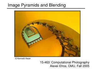
Image Pyramids and Blending. © Kenneth Kwan . 15-463: Computational Photography Alexei Efros, CMU, Fall 2005. Image Pyramids. Known as a Gaussian Pyramid [Burt and Adelson, 1983] In computer graphics, a mip map [Williams, 1983] A precursor to wavelet transform.

E N D
Image Pyramids and Blending © Kenneth Kwan 15-463: Computational Photography Alexei Efros, CMU, Fall 2005
Image Pyramids • Known as a Gaussian Pyramid [Burt and Adelson, 1983] • In computer graphics, a mip map [Williams, 1983] • A precursor to wavelet transform
A bar in the big images is a hair on the zebra’s nose; in smaller images, a stripe; in the smallest, the animal’s nose Figure from David Forsyth
What are they good for? • Improve Search • Search over translations • Like homework • Classic coarse-to-fine strategy • Search over scale • Template matching • E.g. find a face at different scales • Precomputation • Need to access image at different blur levels • Useful for texture mapping at different resolutions (called mip-mapping) • Image Processing • Editing frequency bands separately • E.g. image blending…
Gaussian pyramid construction filter mask • Repeat • Filter • Subsample • Until minimum resolution reached • can specify desired number of levels (e.g., 3-level pyramid) • The whole pyramid is only 4/3 the size of the original image!
Image sub-sampling 1/8 1/4 • Throw away every other row and column to create a 1/2 size image • - called image sub-sampling
Image sub-sampling 1/2 1/4 (2x zoom) 1/8 (4x zoom) Why does this look so bad?
Sampling • Good sampling: • Sample often or, • Sample wisely • Bad sampling: • see aliasing in action!
Input signal: Matlab output: WHY? x = 0:.05:5; imagesc(sin((2.^x).*x)) Aj-aj-aj: Alias! Not enough samples Alias: n., an assumed name Picket fence receding Into the distance will produce aliasing…
Gaussian pre-filtering G 1/8 G 1/4 Gaussian 1/2 • Solution: filter the image, then subsample • Filter size should double for each ½ size reduction. Why?
Subsampling with Gaussian pre-filtering Gaussian 1/2 G 1/4 G 1/8 • Solution: filter the image, then subsample • Filter size should double for each ½ size reduction. Why? • How can we speed this up?
Compare with... 1/2 1/4 (2x zoom) 1/8 (4x zoom)
+ = 1 0 1 0 Feathering Encoding transparency I(x,y) = (aR, aG, aB, a) Iblend = Ileft + Iright
0 1 0 1 Affect of Window Size left right
0 1 0 1 Affect of Window Size
0 1 Good Window Size “Optimal” Window: smooth but not ghosted
Natural to cast this in the Fourier domain • largest frequency <= 2*size of smallest frequency • image frequency content should occupy one “octave” (power of two) FFT What is the Optimal Window? • To avoid seams • window >= size of largest prominent feature • To avoid ghosting • window <= 2*size of smallest prominent feature
FFT What if the Frequency Spread is Wide • Idea (Burt and Adelson) • Compute Fleft = FFT(Ileft), Fright = FFT(Iright) • Decompose Fourier image into octaves (bands) • Fleft = Fleft1 + Fleft2 + … • Feather corresponding octaves Flefti with Frighti • Can compute inverse FFT and feather in spatial domain • Sum feathered octave images in frequency domain • Better implemented in spatial domain
What does blurring take away? original
What does blurring take away? smoothed (5x5 Gaussian)
High-Pass filter smoothed – original
Band-pass filtering • Laplacian Pyramid (subband images) • Created from Gaussian pyramid by subtraction Gaussian Pyramid (low-pass images)
Laplacian Pyramid • How can we reconstruct (collapse) this pyramid into the original image? Need this! Original image
0 1 0 1 0 1 Pyramid Blending Left pyramid blend Right pyramid
laplacian level 4 laplacian level 2 laplacian level 0 left pyramid right pyramid blended pyramid
Laplacian Pyramid: Blending • General Approach: • Build Laplacian pyramids LA and LB from images A and B • Build a Gaussian pyramid GR from selected region R • Form a combined pyramid LS from LA and LB using nodes of GR as weights: • LS(i,j) = GR(I,j,)*LA(I,j) + (1-GR(I,j))*LB(I,j) • Collapse the LS pyramid to get the final blended image
Horror Photo © prof. dmartin
Simplification: Two-band Blending • Brown & Lowe, 2003 • Only use two bands: high freq. and low freq. • Blends low freq. smoothly • Blend high freq. with no smoothing: use binary mask
2-band Blending Low frequency (l > 2 pixels) High frequency (l < 2 pixels)
Gradient Domain • In Pyramid Blending, we decomposed our image into 2nd derivatives (Laplacian) and a low-res image • Let us now look at 1st derivatives (gradients): • No need for low-res image • captures everything (up to a constant) • Idea: • Differentiate • Blend • Reintegrate
Gradient Domain blending (1D) bright Two signals dark Regular blending Blending derivatives
Gradient Domain Blending (2D) • Trickier in 2D: • Take partial derivatives dx and dy (the gradient field) • Fidle around with them (smooth, blend, feather, etc) • Reintegrate • But now integral(dx) might not equal integral(dy) • Find the most agreeable solution • Equivalent to solving Poisson equation • Can use FFT, deconvolution, multigrid solvers, etc.
Perez et al, 2003 • Limitations: • Can’t do contrast reversal (gray on black -> gray on white) • Colored backgrounds “bleed through” • Images need to be very well aligned editing
Don’t blend, CUT! • So far we only tried to blend between two images. What about finding an optimal seam? Moving objects become ghosts
Davis, 1998 • Segment the mosaic • Single source image per segment • Avoid artifacts along boundries • Dijkstra’s algorithm
B1 B1 B2 B2 Neighboring blocks constrained by overlap Minimal error boundary cut Efros & Freeman, 2001 block Input texture B1 B2 Random placement of blocks
2 _ = overlap error min. error boundary Minimal error boundary overlapping blocks vertical boundary
Graphcuts • What if we want similar “cut-where-things-agree” idea, but for closed regions? • Dynamic programming can’t handle loops
a cut hard constraint n-links hard constraint t s Graph cuts (simple example à la Boykov&Jolly, ICCV’01) Minimum cost cut can be computed in polynomial time (max-flow/min-cut algorithms)
Kwatra et al, 2003 Actually, for this example, DP will work just as well…