Download
1 / 29
300 likes | 438 Vues
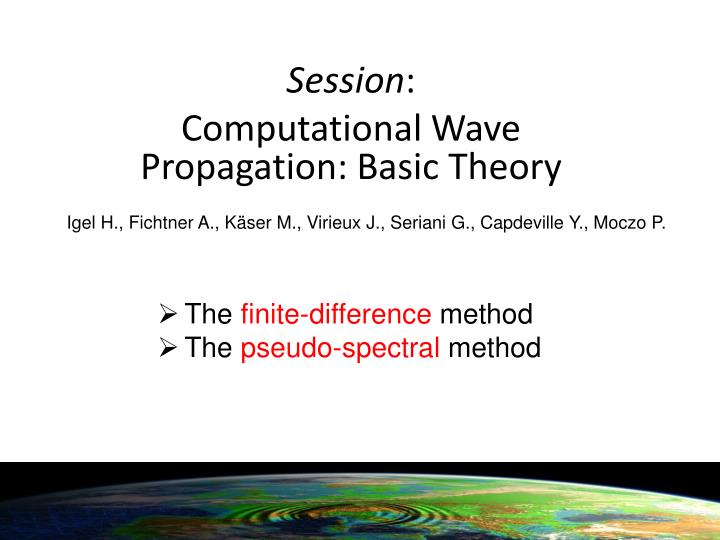
Igel H., Fichtner A., Käser M., Virieux J., Seriani G., Capdeville Y., Moczo P. The finite-difference method The pseudo-spectral method. Session : Computational Wave Propagation: Basic Theory. The problem. The wave equation.

E N D
Igel H., Fichtner A., Käser M., Virieux J., Seriani G., Capdeville Y., Moczo P. • The finite-difference method • The pseudo-spectral method Session: Computational Wave Propagation: Basic Theory
The wave equation Displacement u, elastic parameters E(x) vary only in one direction. Density r and Lame parameters l and m. shear waves P waves with the corresponding velocities shear waves P waves
… we disregard … 3-dimensionality External forces Viscoelastic behaviour Anisotropic behaviour Non-linear elasticity Etc. … and even further simplify and re-write to …
… motion of a string … Displacement u, shear modulus m(x), density r vary only in one direction x.
The velocity-stress formulation stress-strain Generalized Interpolation Low-order to spectral accuracy Extrapolation usually low-order
Other forms of the elastic wave equation Strong form (see Moczo et al.) Displacement – stress Displacement – velocity – stress Velocity – stress Displacement Weak form (more later) Projection on test functions
Numerical methods Finite differences Pseudospectral methods Finite (spectral) elements (Fichtner) Discontinuous Galerkin (Käser) Frequency domain methods (Virieux) Cell methods (Seriani) (Boundary integral methods, lattice solids, discrete wavenumber, finite volumes, etc).
Finite Differences forward difference backward difference centered difference
... or even … … in space and for time … This turns out to be a useful approximation!
Discrete space-time Space and time discretization Regular, 1D
Our first FD wave algorithm Space discretization Regular, 1D
… and the explicit extrapolation scheme … Source term Do for all times … Stop!
… staggered grids … ? the only unknown l+1/2 Time l l-1/2 m-1/2 m m+1/2 Space
Numerical dispersion Amplitude Time
Von Neumann Analysisplane wave analysis continuous discrete Conditional stability
Numerical dispersion phase velocity - group velocity Theoretical prediction of phase and group velocities as a function of wavelength. In 2-D, 3-D this effect depends on direction (-> grid anisotropy)
Well, let us have a closer look at the space derivatives (because there is not so much we can do about the time derivative …)
The pseudospectral approach in the discrete world that means, we can … Discrete Spectrum Exact derivative
PS Algorithm (displacement) Derivatives calculated by DFT (forward and inverse transform and multiplication with –ik) …. cool algorithm, but …
… some more thoughts on the spectral derivative operator „-ik“ … using the convolution theorem … Differential operator in space domain The function we want to differentiate
„Convolution“ d*f f 0 1 0 0 0 d 1 -2 1 0 1 0 0 0 1 -2 1 0 1 0 0 1 1 -2 1 0 1 0 0 -2 1 -2 1 0 1 0 0 1 1 -2 1 0 1 0 0 0 1 -2 1
The numerical wave number as a function of true wave number (ik as a function of k) This is the derivative operater d(x) and it s discrete version (dots)
Finite difference - Pseudospectral nx-point 2-4-6 point Length of (convolutional) operator Increasing accuracy Increasing floating point operations Fourier (Chebysheff) coefficients Taylor coefficients PS FD
FD in real 3-D applications Cartesian Geometry Spherical coordinates Sections Axisymmetric Rheologies Viscolastic Anisotropic Poroelastic Dynamic rupture
Finite Differences - Pros and Cons PROS simple theory Explicit scheme – no matrix inversion Easy parallelization Easy model generation (on regular grids) Easy adaptation to specific problems CONS Boundary conditions difficult to implement Requires large number of grid points per wavelength (in particular surface waves) Large memory requirement Inefficient for models with strong velocity variations Topography not easily implemented
Pseudospectral Method - Pros and Cons PROS Beautiful! Exact space derivatives Explicit scheme – no matrix inversion Centred scheme (anisotropy) Accurate implementation of boundary condition (Chebyshev) Memory efficient (less points per wavelength w.r.t. FD) CONS Global communication scheme (inefficient parallelization) Irregular grid points (Chebyshev) –> stability problems Boundary conditions difficult for Fourier Method
Final thoughts Some of the fundamental concepts of computational seismology can be understood from FD schemes (e.g., stability, dispersion) Each QUEST researcher should be able to Understand what time steps and grid distances are appropriate for a specific Earth velocity models Understand what affects the accuracy of wave simulations (np/l; operators used, wave type, complexity of velocity model, propagation distance, etc.) Know the possible traps of (community) algorithms (black boxes) Know how to benchmark simulation codes (for accuracy)

![G3 - RADIO WAVE PROPAGATION [3 Exam Questions -- 3 Groups]](https://cdn0.slideserve.com/819386/g3-radio-wave-propagation-3-exam-questions-3-groups-dt.jpg)