Download

1 / 15
150 likes | 241 Vues
Lecture 5 Elasticity. Required Text: Frank and Bernanke – Chapter 4. Market Demand Curve. For every single consumer there is a separate demand curve. If we have two consumers in the market, then we will have two individual demand curves, D1 and D2. P. P 1. P 2. D2. D1. Q 1. Q 2. Q.

E N D
Lecture 5Elasticity Required Text: Frank and Bernanke – Chapter 4
Market Demand Curve • For every single consumer there is a separate demand curve. • If we have two consumers in the market, then we will have two individual demand curves, D1 and D2. P P1 P2 D2 D1 Q1 Q2 Q
Market Demand • Given the two demand curves D1 and D2 • Note that , at price=$2, Consumer 1 buys 10 units Consumer 2 buys 20 units Thus the market demand at P=$2 is 30 units • At price=$1, Consumer 1 buys 22 units Consumer 2 buys 30 units. Thus the market demand is 52 units. • Thus, the aggregate or market demand is obtained by the horizontal summation of all individual consumer’s demand curves. P Market Demand $2 $1 D2 D1 10 22 20 30 Q 52
Market Demand • Market Demand - a schedule showing the amounts of a good consumers are willing and able to purchase in the market at different price levels during a specified period of time. • Change in its own price results in a movement along the demand curve. P P1 P2 Market Demand Q1 Q2 Q
Factors that Shift the Market Demand Curve • Population • Tastes • Income • Normal good • Inferior good • Price of Related Goods • Substitutes - increase in the price of a substitute, the demand curve for the related good shifts outward (& vice versa) • Complements - increase in the price of a complement, the demand curve for the related good shifts inward (& vice versa) • Expectations • Expectations about future prices, product availability, and income can affect demand. P D1 D D2 Q
Responsiveness of the Quantity Demanded to a Price Change • Earlier, we indicated that, ceteris paribus, the quantity of a product demanded will vary inversely to the price of that product. That is, the direction of change in quantity demanded following a price change is clear. • What is not known is the extent by which quantity demanded will respond to a price change. • To measure the responsiveness of the quantity demanded to change in price, we use a measure called PRICE ELASTICITY OF DEMAND.
Price Elasticity of Demand (ED) • Price Elasticity of demand for a good is defined as the percentage change in the quantity demanded relative to a percentage change in the good’s own price. Algebraically:
Classifications of Own-Price Elasticity of Demand • Classifications: • Inelastic demand ( |Ed| < 1 ): a change in price brings about a relatively smaller change in quantity demanded (ex. gasoline). • Total Revenue = P×Q rises as a result of a price increase • Unitary elastic demand ( |Ed| = 1 ): a change in price brings about an equivalent change in quantity demanded. • TR= P×Q remains the same as a result of a price increase • Elastic demand ( |Ed| > 1 ): a change in price brings about a relatively larger change in quantity demanded (ex. expensive wine). • TR = P×Q falls as a result of a price increase
Using Price Elasticity of Demand • Elasticity is a pure ratio independent of units. • Since price and quantity demanded generally move in opposite direction, the sign of the elasticity coefficient is generally negative. • Interpretation: If Ed = - 2.72: A one percent increase in price results in a 2.72% decrease in quantity demanded
Price Elasticity along Linear Demand Curves P • Linear Demand Curve: Q = a – bP • Price elasticity of this demand Ed = (∂Q/ ∂P)(P/Q) = − b(P/Q) • Any downward sloping demand curve has a corresponding inverse demand curve. • Inverse linear Demand Curve: P = a/b – (1/b)Q a/b M a/2b Q 0 a/2 a • At P= a/b, Ed = − ∞;atP = 0, Ed = 0; at P= a/2b, Ed = −1 • In the region of the demand curve to the left of the mid-point M, demand is elastic, that is − ∞ ≤ Ed < – 1 • In the region to the right of the mid-point M, demand is inelastic, – 1 < Ed ≤ 0
Cross Price Elasticity of Demand • Shows the percentage change in the quantity demanded of good Y in response to a change in the price of good X. • Edyx = % Change in Qdy / % change in Px • Algebraically: Read as the cross-price elasticity of demand for commodity Y with respect to commodity X. Units of Y demanded Price of X Edyx 60 $10 40 $12 (-20/2)x(10/60) = - 1.66
Classification of Cross-price elasticity of Demand • Interpretation: • If Edyx= - 0.36: A one percent increase in price of chips results in a 0.36% decrease in quantity demanded of beer • Classification: • If (Edyx > 0): implies that as the price of good X increases, the quantity demanded of Good Y also increases. Thus, Y and X are substitutes in consumption (ex. chicken and pork). • If (Edyx < 0): implies that as the price of good X increases, the quantity demanded of Good Y decreases. Thus Y & X are complements in consumption (ex. bear and chips). • If (Edyx = 0): implies that the price of good X has no effect on quantity demanded of Good Y. Thus, Y & X are Independent in consumption (ex. bread and coke)
Income Elasticity of Demand (EI) • Shows the percentage change in the quantity demanded of good Y in response to a percentage change in Income. • EI = % Change in QY / % change in I • Algebraically: Units of Y demanded Income EI 100 $1200 150 $1600 (50/400)x(1200/100) = 1.5
Income Elasticity of Demand (EI) • Interpretation: • If EI= 2.27: A one percent increase income results in a 2.27% increase in quantity demanded of beer • Classification: • If EI> 0, then the good is considered a normal good (ex. beef). • If EI< 0, then the good is considered an inferior good (ex. ramen noodles) • High income elasticity of demand for luxury goods • Low income elasticity of demand for necessary goods
Price Elasticity of Supply (ED) • Price Elasticity of supply of a good is defined as the percentage change in the quantity supplied relative to a percentage change in the good’s own price. Algebraically: • Perfectly inelastic supple – A vertical supply curve • Perfectly elastic supply – a horizontal supply curve.