Download
1 / 22
220 likes | 384 Vues
Non perturbative QCD. ECOLE PREDOCTORALE REGIONALE DE PHYSIQUE SUBATOMIQUE Annecy, 14-18 septembre 2009. Matière atomes électrons protons quarks. Basic notions Path integral Non-perturbative computing methods

E N D
Non perturbative QCD ECOLE PREDOCTORALE REGIONALE DE PHYSIQUE SUBATOMIQUEAnnecy, 14-18 septembre 2009 Matière atomes électrons protons quarks • Basic notions • Path integral • Non-perturbative computing methods • Some applications: beauty physics, form factors, structure functions, finite T, … http://www.th.u-psud.fr/page_perso/Pene/Ecole_predoctorale/index.html
1965 -1975 Quark model Unified Electroweak Theory Strong interaction theory (Quantum Chromodynamics -QCD) Both are quantum field theories, with a gauge invariance. Cabibbo-Kobayashi-Maskawa CP violation mechanism. Successful prediction of a third generation of quarks. Very Well verified by experiment A scientific revolution: The discovery of the standard model However, this is not the last word. There must exist physics beyond the standard model, today unknown: neutrino masses, Baryon number of the universe, electric neutrality of the atom, quantum gravity, … What will we learn from LHC ?
Fundamental Particles + Higgs boson, to be discovered; at LHC ?
QCD: Theory of the strong subnuclear interaction How do quarks and gluons combine to build-up protons, neutrons, pions and other hadrons. Hadronic matter represents 99% of the visible matter of universe How do protons and neutrons combine to Build-up atomic nuclei ?
During the 60’s, understanding strong interactions seemed to be an insurmountable challenge ! and yet, … Beginning of the 70’s QCD was discovered and very fast confirmed by experiment Asplendid scientific epic. cf Patrick Aurenche
Example, the 4 theory: the field is a real function of space-time. Te Lagrangian defines its dynamics (we shall see how): L = 1/2 (∂µ(x))2 -1/2m2 2 (x) - /4! 4(x)The action is defined for all field theory by S=∫d4x L(x) Quantum Field theory (QFT) Lagrange QCD a QFT (synthesis of special relativity and quantum mecanics): We must first define fields and the corresponding particles. We must define the dynamics (the Lagrangian has the advantage of a manifest Lorentz invariance (the Hamiltonien does not) and the symmetries. Last but not least: we must learn how to compute physical quantities. This is the hard part for QCD.
QCD’s Dynamics : Lagrangien Three « colors » a kind of generalised charge related to the « gauge group» SU(3).Action: SQCD=∫d4x LQCD(x)On every space-time point: 3(colors)x6(u,d,s,c,b,t) quarks/antiquark fields [Dirac spinors] q(x) and 8 real gluon fields [Lorentz vectors] Aa(x) - - L = -1/4 GaµGaµ + i∑f qifµ (Dµ)ij qjf -mf qifq if Where a=1,8 gluon colors, i,j=1,3 quark colors, F=1,6 quark flavors, µ Lorentz indices Gaµ=∂µAa- ∂Aaµ+ gfabcAbµ Ac (D µ)ij = ij∂µ - i g aij /2 Aaµ fabcis SU(3)’s structure constant, aij are Gell-Mann matrices q = qt0 -- The Lagrangian of QED is obtained from the same formulae after withdrawing color indices a,b,c,i,j; fabc 0 et aij /21 The major difference is the gluon-gluon interaction
An astounding consequence of this Lagrangian Confinement • One never observes isolated quarks neither gluons. They only exist in bound states, hadrons (color singlets) made up of: • three quarks or three anti-quarks, the (anti-)baryons, example: the proton, neutron, lambda, …. • one quark and one anti-quark, mésons, example: the pion, kaon, B, the J/psi,.. confinement has not yet been derived from QCD Image:we pull afar two heavy quarks, a strong « string » binds them (linear potential). At som point the string breaks, a quark-antiquark pair jumps out of the vacuum to produce two mesons. You never have separated quarks and antiquarks. Imagine you do the same with the electron and proton of H atom. The force is less and at some point e and pare separated (ionisation).
Strong interaction is omnipresent It explains: Hadrons structure and masses The properties of atomic nuclei The « form factors » of hadrons (ex: p+e -> p+e) The final states of p+e -> e+ hadrons (pions, nucleons…) The products of high energy collisions: e- e+ -> hadrons (beaucoup de hadrons) The products of pp-> X (hadrons) Heavy ions collisions (Au + Au -> X), new states of matter (quark gluon plasmas) And all which includes heavier quarks (s,c,b,t) ……….
Apology of QCD Prototype of a « beautiful theory»: Newton’s A « beautiful theory » contains an input precise and condensed, principles, postulates, free parameters (QCD: simple Lagrangian of quarks and gluons, 7 parameters). A very rich output,many physical observables (QCD: millions of experiments implying hundreds of « hadrons »: baryons, mesons, nuclei). QCD is noticeable by the unequated number and variety of its « outputs » Confinement : « input » speaks about a few quarks and gluons, et la « output », hundred’s of hadrons, of nuclei. This metamorphosis is presumably the reason of that rich variety of « outputs ». BUT the accuracy of the predictions is rather low
Jauge 2CV Gauge invarianceredundancy of degrees of freedomdrastically reduces the size of the input, reduces the “ultraviolet” singularities, makes the théory renormalisable • Finite / Infinitesimal : g(x) ≈ exp[ ia(x)a/2] • Huit fonctions réelles a, a=1,8 • Finite gauge transformation A=a Aaa/2 where gauge Invariants Gauge covariant: D g -1(x) D(x)g(x)
Symmetries • Symetric for: • Poincarré invariance • TCP • Charge Conjugation • Chiral (approximate symmetry) • flavour (approximate symmetry) • Heavy quark symmetry (approximate symmetry) • Parity • CP Mystery of strong CP violation, never observed
What to compute and how ? • What objects are we intérested in ? Green functions • What formula allows to compute them ? Path integral • How to tame path integral ? Continuation to imaginary time
Green functions, a couple of examples Quark propagator (non gauge-invariant) S(x,y) is a 12x12 matrix (spin x color) current-current Green function 22 y où Tis gauge-invariant. Im{T} related to the (e+e-hadrons) total cross-section y
Path intégral In a generic quantum field theory, the vacuum expectation value of an operator Ois given by Is a generic bosonic field The action S[] is: R.P.Feynman The « i » in the exponential accounts for quantum interferences between paths. Extremely painful numerically For example the propagator of the particle « » is given by: - The path integral of a fermion wih an action d4xd4y (x)M(x,y) (y) is given by Det[M]
Fermionic Determinants The « quark » part of QCD Lagrangien is Where Mf(x,y) is a matrix in the space direct product of space-time x spin x color The intégral is performed with integration variables defined in Grassman algebra
Path integral of gauge fields Where fixes the gauge: =0,Landau gauge : Is the Faddeev Popov determinant, necessary to protect gauge invariance of the final result SG= -1/4d4x GaµGaµ Flipping to imaginary time
Continuation to imaginary time t =-i, exp[i SG] exp[- SG] SG is positive, exp[-SG]is a probability distribution <O> = ∫DU O exp[- SG]fDet[Mf]/ ∫DU exp[- SG]fDet[Mf] Is a Boltzman distribution in 4 dimensions: exp[- SG] exp[- H] The passage to imaginary time has turned the quantum field theory into a classical thermodynamic theory at equilibrium. The metric becomes Euclidian. Once the Green functions computed with imaginary time, one must return to the quantum field theory, one must perform an analytic continuation in the complex variable faire t or p0. Using the analytic properties of quantum field theory. Simple case, the propagator in time of a particle of energy E: t: real time : imaginary time exp[-iEt] exp[-E] Maupertuis (1744) Maintenant, voici ce principe, si sage, si digne de l'Être suprême : lorsqu'il arrive quelque changement dans la Nature, la quantité d'Action employée pour ce changement est toujours la plus petite qu'il soit possible. »
Suite au prochain épisode
Caractères spéciaux • ∂µ L • L = 1/2 (∂µ(x))2 -1/2m2 2 (x)- /4! 4(x) • L = -1/4 GaµGaµ + i∑f qifµ (Dµ)ijqjf -mf qifq if • Gaµ=∂µAa- ∂Aaµ+ gfabcAbµ Ac • (D µ)ij = ij∂µ - i g aij /2 Aaµ