Download
1 / 19
190 likes | 372 Vues
Meta-population models and movement (Continued). Fish 458; Lecture 19. Modeling Approaches. Discrete areas / grids with exchange (be careful of discrete assumptions). Advection / diffusion models. Occupancy models (a population is either extant or extinct at a given site).

E N D
Meta-population models and movement (Continued) Fish 458; Lecture 19
Modeling Approaches • Discrete areas / grids with exchange (be careful of discrete assumptions). • Advection / diffusion models. • Occupancy models (a population is either extant or extinct at a given site). • Individual-based models.
Advection-Diffusion Modeling(diffusion) • Consider a site x at time t. Let C(x,t) denote the concentration at the point (x,t). • Now consider the total amount of material between x and x+x. • General law: the rate of change of the amount in this interval equals the net rate at which material flows across its boundary (in the positive direction, J(x,t)) plus the net creation of material in the interval, Q(x,t):
Advection-Diffusion Modeling(diffusion) • By the integral mean value theorem: • Dividing by x and taking the limit x0 gives: • Discrete interpretation: the change in the concentration at a site over time is determined by the net amount entering the site plus net production at the site
Advection-Diffusion Modeling(diffusion) • If animals move “randomly”, the net movement will be from areas of high concentration to those of low concentration. • The simplest way to model this is though Fick’s Law: • Substituting into the previous model gives:
Advection-Diffusion Modeling(back to the logistic model) • Now, let us assume that the diffusion rate is a constant, m, and the net production at x0 is: • This leads to: • But for x= t =1 this is the discrete logistic model with migration!
Time for an Example! • Consider a channel (filled with water and of infinite length), assume that some pollutant is dropped in the centre of the channel. • How does the density of pollutant as a function of distance change with time. • This is typical diffusion problem. To solve it, we discretize the diffusion equation and run it forwards.
Pollutants in Channels-II • Note that you need to be very careful when choosing the step sizes (x and t). I used x=1, t=1 and D=0.1.
Pollutants in Channels-III The pollutant diffuses outward from the point source This eventually convergences to a normal distribution Distance
Drunks and Diffusion • Consider a drunk walking down a north-south road. At each time-step, he (she) moves north or south with equal probability. • We can consider the probability distribution for where he (she) is in the road a “concentration” and apply the diffusion model. • Recall “a random walk” leads to a diffusion process.
Drunks and Diffusion(reflective boundary) There are bouncers at either end of the road and if our drunk gets to them, they put him back in the road!
Drunks and Diffusion(reflective boundary) There is a bouncer at one end of the road but the sea at the other (our drunk must be sailor!)
Advection-Diffusion Modeling(Multiple dimensions) • The standard diffusion model can be extended (constant D) into multiple dimensions:
Estimating Movement Rates using Tagging Data • The model and likelihood:
Needs and Assumptions • Needs: • Tagging in all areas. • Tag return rates known from other sources. • Survival rate known from other sources (either from an assessment or the exploitation rate is assumed proportional to fishing effort). • Assumptions: • Usual assumptions of tagging analyses. • Movement rate is independent of density / time / age. • Survival, movement are independent of age / sex, etc.
An Example • Three areas with true migration matrix: M= 0.2yr-1 1000 released in each area. Effort known exactly No non-reporting Recaptures are Poisson.
An Example The fits are very good – unrealistically so!
Reminder • When fitting tagging data, it is often worthwhile assuming a negative binomial likelihood as tagging data are frequently overdispersed (variance larger than the mean with respect to the Poisson).
Readings • Quinn and Deriso (1999); Chapter 10. • Hilborn (1990).