Download
1 / 22
220 likes | 226 Vues
Learn about multiple regression models and how to interpret regression coefficients. Explore common research questions and assumptions of the model.

E N D
Advanced Statistical Methods: Continuous Variableshttp://statisticalmethods.wordpress.com Multiple Regression – Part I tomescu.1@sociology.osu.edu
The Multiple Regression Model Ŷ = a + b1X1 + b2X2 + ... + biXi - this equationrepresents the best prediction of a DV from several continuous (or dummy) IVs; i.e. itminimizes the squared differences btw. Y and Ŷ least square regression Goal: arrive at a set of regression coefficients (bs) for the IVs that bring Ŷs as close as possible to Ys values Regression coefficients: • minimize (the sum of squared) deviations between Ŷ and Y; • optimize the correlation btw. Ŷ and Y for the data set.
Interpretation of Regression Coefficients: a= the estimated value of Y when all independent (exploratory) variables are zero (X1,…i = 0). bimeasures the partial effect of Xi on Y; = effect of one-unit increase in Xi, holding all other independent variables constant. The estimated parameters b1, b2, ..., bi are partial regression coefficients; they are different from regression coefficients for bi-variate relationships between Y and each exploratory variable.
Three criteria for a number of independent (exploratory) variables: (1) Theory (2) Parsimony (3) Sample size
Common Research Questions • Is the multiple correlation between the DV and the IVs statistically significant? • If yes, which IVs in the equation are important, and which not? • Does adding a new IV to the equation improve the prediction of the DV? • Is prediction of a DV from one set of IVs better than prediction from another set of IVs? Multivariate regression also allows for non-linear relationships, by redefining the IV(s): squaring, cubing, .. of the original IV
Assumptions • Random sampling; • DV = continuous; IV(s) variables = continuous (can be treated as such), or dummies; • Linear relationship btw. the DV& the IVs variables (but we canmodel non-linear relations); • Normally distributed characteristics of Y in the population; • Normality, linearity, and homoskedasticity btw. predicted DV scores (Ŷs) and the errors of prediction (residuals) • Independence of errors; • No large outliers
Initial checks 1. Cases-to-IVs Ratio Rule of thumb: N>= 50 + 8*m for testing the multiple correlation; N>=104 + m for testing individual predictors, where m = no. of IVs Need higher case-to-IVs ratio when: • the DV is skewed (and we do not transform it); • a small effect size is anticipated; • substantial measurement error is to be expected 2. Screening for outliers among the DV and the IVs 3. Multicollinearity - too highly correlated IVs are put in the same regression model
4.Assumptions of normality, linearity, and homoskedasticity btw. predicted DV scores (Ŷs) and the errors of prediction (residuals) 4.a. Multivariate Normality • each variable & all linear combinations of the variables are normally distributed; • if this assumption is met residuals of analysis = normally distributed & independent For grouped data: assumption pertains to the sampling distribution of means of variables; Central Limit Theory: with sufficiently large sample size, sampling distributions are normally distributed regardless of the distribution of the variables What to look for (in ungrouped data): • is each variable normally distributed? Shape of distribution: skewness & kurtosis. Frequency histograms; expected normal probability plots; detrend expected normal probability plots • are the realtionships btw. pairs of variables (a) linear, and (b) homoskedastic (i.e. the variance of one variable is the same at all values of other variables)?
Homoskedasticity • for ungrouped data: the variability in scores for one continuous variable is ~ the same at all values of another continuous variable • for grouped data: the variability in the DV is expected to be ~ the same at all levels of the grouping variable Heteroskedasticity = caused by: • non-normality of one of the variables; • one variable is related to some transformation of the other; • greater error of measurement at some level of an IV
Residuals Scatter Plots to check if: 4.a. Errors of prediction are normally distributed around each & every Ŷ 4.b. Residuals have straight line relationship with Ŷs - If genuine curvilinear relation btw. an IV and the DV, include a square of the IV in the model 4.c. The variance of the residuals about Ŷs is ~the same for all predicted scores (assumption of homoskedasticity) - heteroskedasticity may occur when: - some of the variables are skewed, and others are not; may consider transforming the variable(s) - one IV interacts with another variable that is not part of the equation 5. Errors of prediction are independent of one another Durbin-Watson statistic = measure of autocorrelation of errors over the sequence of cases; if significant it indicates non-independence of errors
Major Types of Multiple Regression Standard multiple regression Sequential (hierarchical) regression Statistical (stepwise) regression R² = a + b + c + d + e R²= the squared multiple correlation; it is the proportion of variation in the DV that is predictable from the best linear combination of the IVs (i.e. coefficient of determination). R = correlation between the observed and predicted Y values (R = ryŶ ) a x2
Adjusted R2 Adjusted R2 = modification of R2 that adjusts for the number of terms in a model. R2 always increases when a new term is added to a model, but adjusted R2 increases only if the new term improves the model more than would be expected by chance.
Standard (Simultaneous) Multiple Regression • all IVs enter into the regression equation at once; each one is assessed as if it had entered the regression after all other IVs had entered. • each IV is assigned only the area of its unique contribution; • the overlapping areas (b & d) contribute to R² but are not assigned to any of the individual IVs
Table 1: Regression of (DV) Assessment of Socialism in 2003 on (IVs) Social Status, controlling for Gender and Age **p <0.001; *p < 0.05; Interpretation of beta (standardized) coefficients: for a one standard deviation unit increase in X, we get a Beta standard deviation change in Y; Since variables are transformed into z-scores (i.e. standradized), we can assess their relative impact on the DV (assuming they are uncorrelated with each other)
Sequential (hierarchical) Multiple Regression - researcher specifies the order in which IVs are added to the equation; • each IV/IVs are assessed in terms of what they add to the equation at their own point of entry; • If X1 is entered 1st, then X2, then X3: X1 gets credit for a and b; X2 for c and d; X3 for e. IVs can be added one at a time, or in blocks a
The Regression SUM of SQUARES, SS(regression) = SS(total) + SS(residual)SSregression = Sum (Ŷ – Ybar)² = portion of variation in Y explained by the use of the IVs as predictors; SStotal = Sum (Y- Ybar)²SSresidual = Sum (Y- Ŷ)² - the squared sum of errors in predictionsR² = SSreg/SStotal
ANOVA The Regression MEAN SQUARE : MSS(regression) = SS(regression) / df, df = k where k = no. of variables The MEAN square residual (error): MSS(residual) = SS(residual) / df, df= n - (k + 1) where n = no. of cases and k= no. of variables.
Hypothesis Testing with (Multiple) Regression F – test The null hypothesis for the regression model: Ho: b1 = b2 = … = bk = 0 MSS(model) • F = -------------- MSS(residual) The sampling distribution of this statistic is the F-distribution
t – test for the effect of each independent variable The Null Hypothesis for individual IVs The test of H0: bi = 0 evaluates whether Y and X are statistically dependent, ignoring other variables. We use the t statistic b • t = -------------- σB where σB is a standard error of B SS(residual) • σB = -------- n - 2
Assessing the importance of IVs • if IVs are uncorrelated w. each other: compare standardized coefficients (betas); higher absolute values of betas reflect greater impact; • if the IVs are correlated w. each other: compare total relation of the IV with the DV, and of IVs with each other using bivariate correlations; compare the unique contribution of an IV to predicting the DV = generally assessed through partial or semi-partial correlations In partial correlation (pr), the contribution of the other IVs is taken out of both the IV and the DV; In semi-partial correlation (sr), the contribution of the other IVs is taken out of only the IV (squared) sr shows the unique contribution of the IV to the total variance of the DV
Assessing the importance of IVs – continued In standard multiple regression, sr² = the unique contribution of the IV to R²in that set of IVs (for an IV, sr² = the amount by which R² is reduced, if that IV is deleted from the equation) If IVs are correlated: usually, sum of sri² < R² • the difference R² - sum of sri² for all IVs = shared variance (i.e. variance contributed to R² by 2/more variables) Sequential regression: sri² = amount of variance added to R² by each IV at the point that it is added to the model In SPSS output sri² is „R² Change” for each IV in „Model Summary” Table