Download
1 / 27
270 likes | 505 Vues
Topics in Multivariate Approximation and Interpolation. Parameterization for Curve Interpolation. Michael S. Floater and Tatiana Surazhsky. Speaker: CAI Hong-jie Date: Oct. 11, 2007. The First Author. Michael S. Floater Main Posts Professor of the University of Oslo

E N D
Topics in Multivariate Approximation and Interpolation Parameterization for Curve Interpolation Michael S. Floater and Tatiana Surazhsky Speaker: CAI Hong-jie Date: Oct. 11, 2007
The First Author Michael S. Floater • Main Posts Professor of the University of Oslo Editor of the journal Computer Aided Geometric Design • Research Geometric modeling Numerical analysis Approximation theory
The Second Author Tatiana Surazhsky • Post 3D Researcher of Samsung Electronics, Samsung Telecom Research Israel • Research Geometric modeling Computer graphics
Outline • Background • Metric for approximation error • Approximation order • Cubic polynomial • Cubic spline • higher degree polynomial • Hermite interpolation
P1 Pn P0 Pn-1 Background • Concept: Parameterization for interpolation • Given points P0,P1,…,Pn in Rk, k= 2 or 3 • To find t0<t1<…<tn and parametric curve P(t) such that P(ti)=Pi, i=0,…,n.
Background • Selection of parametric curve • Polynomial curve • Spline curve • Selection of knot vector To determine di:=ti+1-ti, i=0,1,…,n-1.
Choices for di • Uniform di = 1 • Chordal di = |Pi+1-Pi| • J. H. Ahlberg, E. N. Nilson, and J. L. Walsh The theory of splines and their applications, 1967 • M. P. Epstein On the influence of parametrization in parametric interpolation, 1976 • Centripetal di = |Pi+1-Pi|1/2 • E. T. Y. Lee Choosing nodes in parametric curve interpolation, 1989 • Affine invariant • T. A. Foley and G. M. Nielson Knot selection for parametric spline interpolation, 1989
Comparison of Four Choices Original Curve: thin black Spline Curves: thick gray
Comparison of Three Choices Original curve: blue uniform: green Chordal: black centripetal: magenta
Comparison of Three Choices Original curve: blue uniform: green Chordal: black centripetal: magenta
Metric for Approximation Error • Hausdorff distance Let A,B be point sets in Rk (k=2,3), define where ||·||EisEuclidean distance, then Hausdorff distance between A and B is
Metric for Approximation Error • Illustration for Hausdorff distance d(A,B)=1 d(B,A)=3 dH(A,B)=3 • Application of Hausdorff distance Image matching
Hausdorff distance for curves • Definition P0,P1,…,Pnsampled from parametric curve f:[a,b]→ Rk, Pi= f(si), a≤s0<s1<…< sn≤b. Interpolate Piby P(t):[t0,tn]→ Rk, then the distance between them is
Metric for Approximation Error • Parametric distance where Ф: [t0,tn] →[s0,sn] is strictly increasing, C1 functions such that Ф(t0)=s0, Ф(tn)=sn. T. Lyche and K. MØrken, A metric for parametric approximation, Curves and Surfaces, 1994
Approximation Order • Why not distances • Hard to calculate • Even bounds are difficult to achieve • Approximation order instead where h= Length(f| [s0,sn] )= sn-s0. Larger approximation order m, better interpolation
Cubic Polynomial Interpolation • Theorem Givenf∈C4[a,b], samples a≤s0<s1<s2<s3≤b, let t0=0, ti+1- ti=|f(si+1) - f(si)|(i=0,1,2), and P(t):[t0,t3] → Rkbe cubic polynomial such that P(ti)=f(si),i=0,1,2,3. Then dP(f|[s0,s3], P)=O(h4),h→0, where h=s3-s0.
Cubic Polynomial Interpolation • Lemma 1 If f∈C2[a,b], then Tip for proof: let u=(si+si+1)/2, then
Cubic Polynomial Interpolation • Lemma 2 If Ф:[t0, t3] →R cubic polynomial such that Ф(ti)=si, i = 0,1,2,3, then Tip for proof: Newton interpolation formula
Extension to Cubic Spline • Theorem Givenf∈C4[a,b], samples a≤s0<…<sn≤b, let t0=0, ti+1- ti=|f(si+1) - f(si)|, 0 ≤i<n, and σ(t):[t0,tn] → Rkbe the cubic spline curve such that Then dP(f|[s0,sn], σ)=O(h4),h→0, where
Parameterization Improvement for higher degree • Case: polynomial degree n=2,3 • Uniform O(h2) • Chordal O(hn+1) • Case: polynomial degree n= 4,5 • Uniform O(h2) • Chordal O(h4) • Improvement O(hn+1) di=Length(chordal cubic polynomial between Pi,Pi+1)
Hermite Interpolation • Cubic two-point Givenf∈C4[a,b], t1- t0=|f(s1) - f(s0)|, and let P(t):[t0,t1] → Rkbe cubic polynomial such that Then dP(f|[s0,s1], P)=O(h4), as h→0.
Hermite Interpolation • Quintic two-point Givenf∈C6[a,b], let u0, u1 be chordal parametric knot vector, and t0, t1 be improved knot vector, P(t):[t0,t1] → Rkbe quintic polynomial such that Then dP(f|[s0,s1], P)=O(h6), as h→0.
Numerical Examples Original curve
Comparison with Cubic Spline • Samples from a glass cup • Chordal C2 cubic spline curve • Improved C2quintic Hermite spline curve
Reference • M.S. Floater ,T. Surazhsky. Parameterization for curve interpolation. Topics in Multivariate Approximation and Interpolation, 2007. • M.S. Floater. Arc Length Estimation and The Convergence of Polynomial Curve Interpolation. Numerical Mathematics, to appear. • T. Surazhsky, V. Surazhsky. Sampling Planar Curves Using Curvature-Based Shape Analysis. Mathematical Methods for Curves and Surfaces, Tromsø 2004. • 李庆杨,王能超,易大义. 数值分析,第4版,2003.