Download
1 / 23
230 likes | 252 Vues
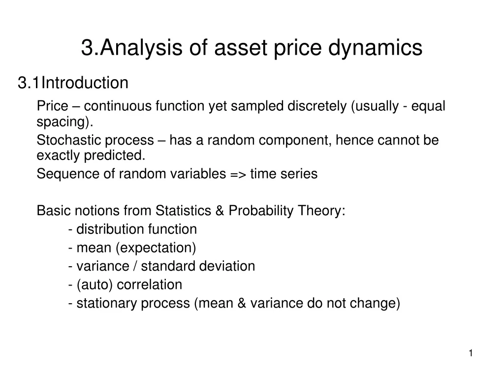
3.Analysis of asset price dynamics. 3.1Introduction Price – continuous function yet sampled discretely (usually - equal spacing). Stochastic process – has a random component, hence cannot be exactly predicted. Sequence of random variables => time series

E N D
3.Analysis of asset price dynamics 3.1Introduction Price – continuous function yet sampled discretely (usually - equal spacing). Stochastic process – has a random component, hence cannot be exactly predicted. Sequence of random variables => time series Basic notions from Statistics & Probability Theory: - distribution function - mean (expectation) - variance / standard deviation - (auto) correlation - stationary process (mean & variance do not change)
Statistical concepts 1 • Consider a random variable (or variate) X. Probability density functionf(x) defines the probability to find X between a and b: Pr(a≤ X ≤ b) = The probability density must satisfy the normalization condition = 1 • Cumulative distribution function: Pr(X≤b) = Obviously, Pr(X > b) = 1 – Pr(X ≤ b)
Statistical concepts 2 • Two characteristics are used to describe the most probable values of random variables: (1) mean (or expectation), and (2) median. Mean of X is the average of all possible values of X that are weighed with the probability density f(x): m= E[X] = ∫ x f(x)dx Median of X is the value M for which Pr(X> M) = Pr(X < M) = 0.5 • Variance, Var, and thestandard deviation,σ, are the conventional estimates of the deviations from the mean values of X Var[X] ≡ σ2 = ∫(x – m)2f(x) dx
Statistical concepts 3 Higher-order moments of the probability distributions are defined as mn= E[Xn] = ∫ xn f(x) dx According to this definition, mean is the first moment (m ≡ m1), and variance can be expressed via the first two moments, σ2 = m2 – m2. Two other important parameters,skewnessS and kurtosisK, are related to the third and fourth moments, respectively: S= E[(x – m)3] / σ3 , K = E[(x – m)4] / σ4 Both Sand K are dimensionless. Zero skewness implies that f(x) is symmetrical around its mean value. The positive and negative values of skewness indicate long positive tails and long negative tails, respectively. Kurtosis characterizes the distribution peakedness. Kurtosis of the normal distribution equals three. The excess kurtosis, Ke = K – 3, is often used as a measure of deviation from the normal distribution.
Statistical concepts 4 • Joint distribution of two random variables X and Y Pr(X≤ b, Y ≤ c) = h(x, y) is the joint density that satisfies the normalization condition =1 Two random variables are independent if their joint density function is the product of the univariate density functions: h(x, y) = f(x) g(y). • Covariance between two variates provides a measure of their simultaneous change. Consider two variatesX and Y that have the means mX and mY, respectively. Their covariance equals Cov(x, y) = σXY = E[(x –mX)(y – mY)] = E[xy] – mXmY
Statistical concepts 5 Positive (negative) covariance between two variates implies that these variates tend to change simultaneously in the same (opposite) direction. • Another popular measure of simultaneous change is correlation coefficient: Corr(x, y) = Cov(x, y)/(σXσY); -1 ≤ Corr(x, y) ≤ 1 • Autocovariance: γ(k, t) = E[y(t) – m)(y(t – k) – m)] • Autocorrelation function (ACF): ρ(k) = γ(k)/γ(0); ρ(0) = 1; |ρ(k)| < 1 • Ljung-Box test H0 hypothesis: ρ(1) = ρ(2) = … ρ(k) = 0; p-value. In the general case with NvariatesX1, . . ., XN(where N > 2), correlations among variates are described with the covariance matrix, which has the following elements Cov(xi, xj) = σij = E[(xi – mi)(xj – mj)]
Statistical concepts 6 • Uniform distribution has a constant value within the given interval [a, b] and equals zero outside this interval fU= 0, x < a and x > b fU= 1/(b – a), a ≤ x ≤ b mU= 0.5(a+b), σ2U = (b – a)2/12, SU = 0, KeU = –6/5 • Normal (Gaussian) distribution has the form fN(x) = exp[–(x – m)2/2σ2] It is often denoted N(m, σ). Skewness and excess kurtosis of the normal distribution equal zero. The transform z = (x – m)/σ converts the normal distribution into the standard normal distribution fSN(x) = exp[–z2/2]
Statistical concepts 7 Estimation for a given data sample Sample mean: m = Sample variance: σ2 = - m)2 Sample standard error: SE =
3.Analysis of asset price dynamics 3.1Introduction (continued) Time series analysis: - ARMA model - linear regression - trends (deterministic vs stochastic) - vector autoregressions /simultaneous equations - cointegration 9
3.Analysis of asset price dynamics 3.2 Autoregressive model AR(p) Univariate time series y(t) observed at moments t = 0, 1, …, n; y(tk) ≡ y(k) ≡ yk y(t) = a1y(t-1) + a2y(t-2) + …+ apy(t-p) + ε(t), t > p (lag) Random process ε(t) (noise, shock, innovation) White noise: E[ε(t)] = 0; E[ε2(t)] = 2; E[ε(t) ε(s)] = 0, if ts. Lag operator: Lp = y(t-p); Ap(L) = 1 – a1L – a2L2 - … - apLp AR(p): Ap(L)y(t) = ε(t), 10
3.Analysis of asset price dynamics 3.2 Autoregressive model AR(p) (continued 1) AR(1): y(t) = a1y(t-1) + ε(t), y(t) = a1iε(t-i) Mean-reverting process: shocks decay and process returns to its mean. “Old” noise converges with time to zero when | a1| < 1 If a1= 1, AR(1) is the random walk (RW): y(t) = y(t-1) + ε(t) => y(t) = ε(t-i) RW is not mean-reverting. 11
3. Analysis of asset price dynamics 3.2 Autoregressive model AR(p) (continued 2) The 1st difference of RW: x(t) = y(t) – y(t-1) = ε(t) => mean-reverting Processes that must be differenced d times in order to exclude non-transitory noise shocks are named integratedof order d: I(d). Unit roots exist for AR(p) when shocks are not transitory. Then modulus of solutions to the characterisitc equation 1 – a1z – a2z2 - … - apzp = 0 must be lower than 1 (inside unit circle): y(t) = 0.5y(t-1) – 0.2y(t-2) => 1- 0.5z + 0.2z2 = 0;
3. Analysis of asset price dynamics 3.2 Autoregressive model AR(p) (continued 3) AR(p) with non-zero mean: If E[y(t)] = m, RW: y(t) = c + a1y(t-1) + ε(t), c = m(1- a1) AR(p): Ap(L)y(t) = c + ε(t), c = m(1- a1 - ... - ap) Autocorrelation coefficients: y(t) is covariance-stationary (or weakly stationary) if γ(k, t) = γ(k). AR(1): ρ(1) = a1 , ρ(k) = a1ρ(k-1) AR(2): ρ(1) = a1/(1 – a2), ρ(k) = a1ρ(k-1) + a2ρ(k-2), k ≥ 2
3. Analysis of asset price dynamics 3.3 Moving average model MA(q) y(t) = ε(t) + b1ε(t-1) + b2ε(t-2) + ... + bqε(t-q) = Bq(L) ε(t) Bq(L) = 1 + b1L + b2L2 + … + bqLq MA(1): y(t) = ε(t) + b1ε(t-1), ε(0) = 0; MA(1) incorporates past like AR(): y(t)(1-b1L + b1L2-b1L3+ ...) = ε(t) MA(1): ρ(1) = b1/( b12 + 1) , ρ(k>1) = 0 MA(q) is invertible if it can be transformed into AR(). In this case, all solutions to 1 + b1z + b2z2 + … + bq zq = 0 must be outside unit circle. Hence MA(1) is invertible when |b1|< 1. MA(q) with non-zero mean m: y(t) = c + Bp(L)ε(t), c = m
3. Analysis of asset price dynamics 3.4 The ARMA(p, q) model y(t) = a1y(t-1) + a2y(t-2) + …+ apy(t-p) + ε(t) + b1ε(t-1) + b2ε(t-2) + ... + bqε(t-q) Strict stationarity when higher moments do not depend on time. Any MA(q) is covariance-stationary. AR(p) is covariance-stationary only if the roots of its polynomial are outside the unit circle.
3. Analysis of asset price dynamics 3.5 Linear regression Empirical TS: yi = a + bxi + εi., i = 1, 2, .., N. a – intercept; b – slope. Estimator: y = A + Bx; Residual: ei = yi - A - Bxi; RSS = MSE => OLS = min(RSS) => A = ym - Bxm ; B = xm = ; ym = Xi = xi – xm Yi = yi – ym 16
3. Analysis of asset price dynamics 3.5 Linear regression (continued) Assumptions: 1) E[εi] = 0; otherwise intercept is biased. 2) Var(εi) = σ2 = const ; 3) E[ε(t) ε(s)] = 0, if ts. 4) Independent variable is deterministic. Goodness of fit (coefficient of determination; R2) R2 = 1 -
3. Analysis of asset price dynamics 3.5 Linear regression (continued)
3.Analysis of asset price dynamics 3.6 Multiple regression yi = a + b1x1,i + b2x2,i +... + bKxK,i + εi Additional assumption: no perfect collinearity, i.e. no Xi is a linear combination of other Xi. Overspecification => no bias in estimates of bi but overstates σ2 Underspecification => yields biased bi and understates σ2 Adjusted R2= 1 -
3. Analysis of asset price dynamics 3.7 Trends Trends => non-stationary time series Deterministic trend vs stochastic trend AR(1): y(t) – m – ct = a1[y(t – 1) – m – c(t – 1)] + ε(t) z(t) = y(t) – m – ct= a1tz(0) +ε(t) If |a1| < 1, shocks are transitory. If a1=1, random walk with drift: y(t) = c + y(t – 1) + ε(t) For m=0, deterministic trend: y(t) = at + ε(t) stochastic trend: y(t) = a + y(t – 1) + ε(t) May look similar for some time.
3. Analysis of asset price dynamics 3.8 Multivariate time series A multivariate time series y(t) = (y1(t), y2(t),..., yn(t))' is a vector of n processes Multivariate moving average models are rarely used. Therefore we focus on the vector autoregressive model (VAR). Bivariate VAR(1) process: y1(t) = a10 + a11y1(t - 1) + a12y2(t - 1) + ε1(t) y2(t) = a20 + a21y1(t - 1) + a22y2(t - 1) + ε2(t) Matrix form: y(t) = a0 + Ay(t - 1) + ε(t) y(t) = (y1(t), y2(t))', a0 = (a10, a20)', ε(t) = (ε1(t), ε2(t))', A =
3. Analysis of asset price dynamics 3.9 Multivariate time series (continued) Simultaneous dynamic models y1(t) = a11y1(t - 1) + a12y2(t) + ε1(t) y2(t) = a21y1(t) + a22y2(t - 1) + ε2(t) can be transformed to VAR: = (1 - a12 a21)-1 + (1 - a12 a21)-1 Two covariance stationary processes are x(t) and y(t) are jointly covariance-stationary if Cov(x(t), y(t – s)) depends on lag s only.