Neutron Drip Line in Ca Region: Bayesian Machine Learning

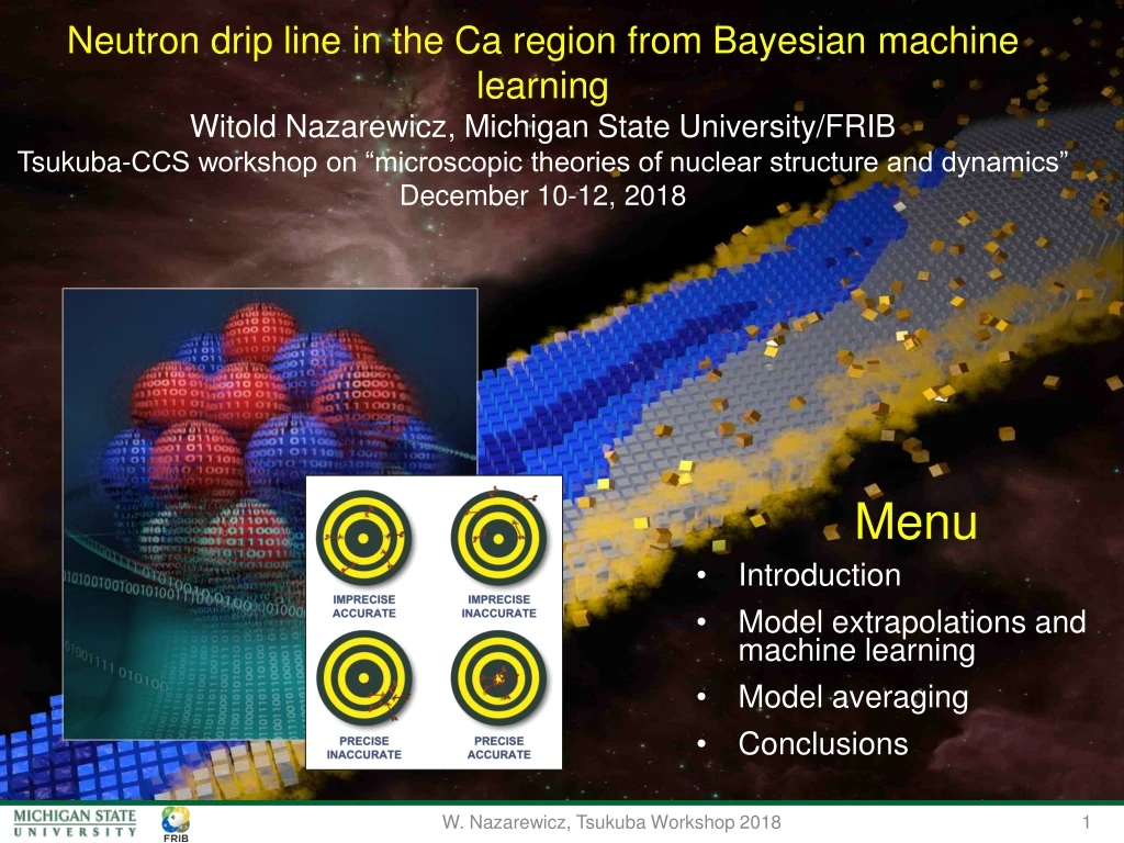
1. Neutron drip line in the Ca region from Bayesian machine learning WitoldNazarewicz, Michigan State University/FRIB Tsukuba-CCS workshop on “microscopic theories of nuclear structure and dynamics” December 10-12, 2018 • Menu • Introduction • Model extrapolations and machine learning • Model averaging • Conclusions W. Nazarewicz, Tsukuba Workshop 2018

2. In many cases, nuclear input MUST involve massive extrapolations based on predicted quantities. And extrapolations are tough. W. Nazarewicz, Tsukuba Workshop 2018

3. Some relevant references… • S. Athanassopoulos, E. Mavrommatis, K. Gernoth, and J. Clark, Nucl. Phys. A 743, 222 (2004). • R. Utama, J. Piekarewicz, and H. B. Prosper, Phys. Rev. C 93, 014311 (2016). • G. F. Bertsch and D. Bingham, Phys. Rev. Lett. 119, 252501 (2017). • H. F. Zhang et al.,J. Phys. G 44, 045110 (2017). • Z. Niu and H. Liang, Phys. Lett. B 778, 48 (2018). • R. Utama and J. Piekarewicz, Phys. Rev. C 97, 014306 (2018). W. Nazarewicz, Tsukuba Workshop 2018

4. Separation energy residual: emulator of residual W. Nazarewicz, Tsukuba Workshop 2018

5. We consider 12 global nuclear mass models: • FRDM-2012, HFB-24: rms mass deviation ~0.6 MeV • SkM*, SkP, SLy4, SV-min, UNEDF0, UNEDF1: 1.5-6 MeV • NL3*, DD-ME2, DD-PC1, DDMEd: 2-3 MeV • The emulators of S2n residuals and confidence intervals defining theoretical error bars are constructed using Bayesian Gaussian processes and Bayesian neural networks. • By establishing statistical methodology and parameters, we carried out extrapolations towards the 2n dripline. W. Nazarewicz, Tsukuba Workshop 2018

6. Our objective: extrapolations We consider a large training dataset pertaining to nuclei whose masses were measured before 2003. For the testing datasets, we considered those exotic nuclei whose masses have been determined after 2003. Training set: 537 points Testing sets: 55+4 points W. Nazarewicz, Tsukuba Workshop 2018

7. Residuals exhibit local trends • This information can be used to our advantage to improve model-based predictions! • It can also be used to improve models themselves W. Nazarewicz, Tsukuba Workshop 2018

8. Bayesian approach residual (Z,N)i Bayes’ theorem Prediction of unknown observable y* given known data y • Two statistical models used: • Gaussian process (3 parameters) • Bayesian neural network with sigmoid function (30 neurons, 1 layer; 181 parameters) • 100,000 iterations of an ergodic Markov chain produced by the Metropolis-Hastings algorithm • Some refinements added based on our knowledge of trends W. Nazarewicz, Tsukuba Workshop 2018

9. GP BNN training dataset: AME2003 testing dataset: AME2016-AME2003 Overall, for the testing dataset AME2016-2003, the rms deviation from experimental S2n values is 400-500 keV in the GP variant for all theoretical models employed in our study, which suggests that our statistical methods capture most of the residual structure. BUT the predicted mean value is certainly not the whole story! W. Nazarewicz, Tsukuba Workshop 2018

10. W. Nazarewicz, Tsukuba Workshop 2018

11. model: N*=126 model+GP: N*=126 (N*=122 at 1s and N*=118 at 1.65s one-sided/credibility 95%) model+BNN: N*=118 (N*=104 at 1s and N*=102 at 1.65s) Can one say: “DD-PC1 predicts the 2n dripline at N=126” ? W. Nazarewicz, Tsukuba Workshop 2018

12. Massive MCMC runs: BNN shows convergence issues! W. Nazarewicz, Tsukuba Workshop 2018

13. Discovery of 60Ca O.B. Tarasov et al. Phys. Rev. Lett. 121, 022501 (2018) 59K ? The eight new neutron-rich nuclei discovered, 47P, 49S, 52Cl, 54Ar, 57K, 59,60Ca, and 62Sc, are the most neutron-rich isotopes of the respective elements. In addition, one event consistent with 59K was registered. W. Nazarewicz, Tsukuba Workshop 2018

14. S. R. Stroberg et al. W. Nazarewicz, Tsukuba Workshop 2018

15. Phys. Scripta 2013, 014022 (2013) W. Nazarewicz, Tsukuba Workshop 2018

16. Validation: new masses of 55-57Ca S. Michimasa, et al., Phys. Rev. Lett. 121, 022506 (2018) W. Nazarewicz, Tsukuba Workshop 2018

17. Probability of existence Neufcourt, Cao, Nazarewicz, Olsen, to be published We introduce the posterior probability pex(Z,N) of the predicted separation energy S1n/2n(Z,N) being positive: * W. Nazarewicz, Tsukuba Workshop 2018

18. Neutron drip line in the Ca region from Bayesian machine learning and Bayesian model averaging W. Nazarewicz, Tsukuba Workshop 2018

19. W. Nazarewicz, Tsukuba Workshop 2018

20. Naïve nuclear theorist’s approach to a systematic (model) error estimate: • Take a set of reasonable global models Mi, hopefully based on different assumptions/formalism, that satisfy basic theoretical requirements (here comes the expert belief thing) • Make predictions: E(y;Mi)=yi • Compute average and variation within this set • Compute rms deviation from existing experimental data. Can we do better? Yes! W. Nazarewicz, Tsukuba Workshop 2018

21. Bayesian model mixing Our model mixing calculations were done by averaging posteriors obtained with individual models. In the first averaging variant, we assumed model-independent prior weights. In the secondposterior averaging variant, the weights were obtained as the Bayesian posterior probabilities that a model Mk predicts the existence of the key nuclei 52Cl, 53Ar, and 49S, namely: W. Nazarewicz, Tsukuba Workshop 2018

22. W. Nazarewicz, Tsukuba Workshop 2018

23. Summary While both Gaussian processes and Bayesian neural networks reduce the rms deviation from experiment significantly, GP offers a better and more stable performance. The increase in the predictive power of DFT models aided by the statistical treatment is quite astonishing: the resulting rms deviations from experiment on the testing dataset are similar to those of well-fitted mass models. The estimated confidence intervals on predictions make it possible to evaluate predictive power of individual models, and also use groups of models to make quantified predictions. We quantified the neutron-stability of the nucleus in terms of its existence probability pex. Our results are fairly consistent with recent experimental findings: 60Ca is expected to be well bound with S2n~ 5 MeV while 49S, 52Cl, and 53Ar are predicted to be marginally-bound threshold systems. One event consistent with 59K was registered. According to our calculations, this nucleus is expected to be firmly neutron-bound. W. Nazarewicz, Tsukuba Workshop 2018

24. Thank you! W. Nazarewicz, Tsukuba Workshop 2018

25. What is required? • Common dataset Y (as large as possible) needs to be defined • Statistical analysis for individual models needs to be carried out (parameter posteriors determined) • Individual model predictions carried out, including statistical uncertainties • Decision should be made on the prior model probability p(Mk) M1 M1271 M2 The posterior mean and variance of y are: Y M3 Ma Ya Y ⊂Ya⊂Ytot set of observables Ytot W. Nazarewicz, Tsukuba Workshop 2018

26. Bayesian Model Averaging (BMA) models considered posterior distribution given data Posterior distribution of y under each model quantity of interest observables (data) posterior probability of a model The posterior probability for the model Mk prior probability that the model Mk is true (!!!) marginal density of the data; integrated likelihood of model Mk prior distribution of parameters likelihood W. Nazarewicz, Tsukuba Workshop 2018

27. Model selection and Bayes Factor (BF) BF an be used to decide which of two models is more likely given a result y. The outcome The posterior mean and variance of y are: W. Nazarewicz, Tsukuba Workshop 2018

28. Bayesian inference & RNB science Beam time and compute cycles are difficult to get and expensive • What is the information content of measured observables? • Are estimated errors of measured observables meaningful? • What experimental data are crucial for better constraining current nuclear models? New technologies are essential for providing predictive capability, to estimate uncertainties, and to assess extrapolations • Theoretical models are often applied to entirely new nuclear systems and conditions that are not accessible to experiment Statistical tools can help us revealing the structure of our models • Parameter reduction • Uncertainty quantification W. Nazarewicz, Tsukuba Workshop 2018

29. From Hoeting and Wasserman: • When faced with several candidate models, the analyst can either choose one model or average over the models. Bayesian methods provide a set of tools for these problems. Bayesian methods also give us a numerical measure of the relative evidence in favor of competing theories. • Model selection refers to the problem of using the data to select one model from the list of candidate models. Model averaging refers to the process of estimating some quantity under each model and then averaging the estimates according to how likely each model is. • Bayesian model selection and model averaging is a conceptually simple, unified approach. An intrinsic Bayes factor might also be a useful approach. • There is no need to choose one model. It is possible to average the predictions from several models. • Simulation methods make it feasible to compute posterior probabilities in many problems. • It should be emphasized that BMA should not be used as an excuse for poor science... BMA is useful after careful scientific analysis of the problem at hand. Indeed, BMA offers one more tool in the toolbox of applied statisticians for improved data analysis and interpretation. W. Nazarewicz, Tsukuba Workshop 2018