Speech Recognition

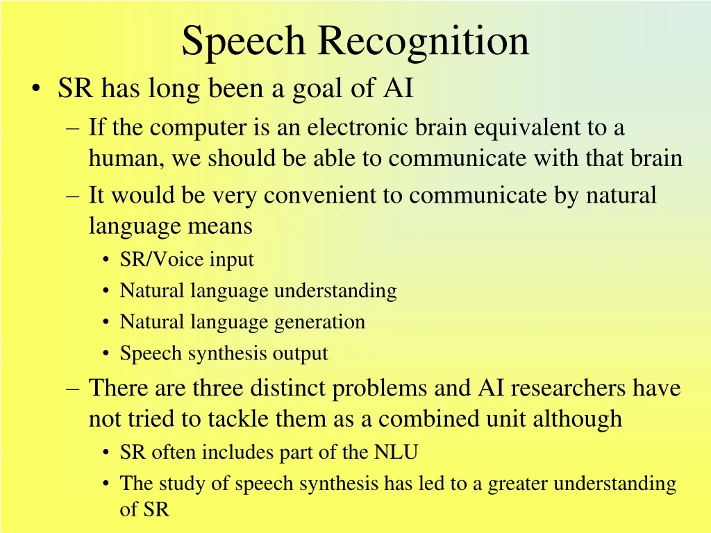
1. Speech Recognition • SR has long been a goal of AI • If the computer is an electronic brain equivalent to a human, we should be able to communicate with that brain • It would be very convenient to communicate by natural language means • SR/Voice input • Natural language understanding • Natural language generation • Speech synthesis output • There are three distinct problems and AI researchers have not tried to tackle them as a combined unit although • SR often includes part of the NLU • The study of speech synthesis has led to a greater understanding of SR

2. Speech Recognition as a Problem • We find a range of possible parameters for the speech recognition task • Speaking mode: isolated words to continuous speech • Speaking style: read speech to conversational (spontaneous) speech • Dependence: speaker dependent (specifically designed for one speaker) to speaker independent trained to speaker independent untrained • Vocabulary: small (50 words or less), moderate (50-200 words), large (1000 words), very large (5000 words), realistic (entire language) • Language model: finite state (HMM, Bayes network), knowledge base, neural network, other • Grammar: bigram/trigram, limited syntax, unlimited syntax • Semantics: small lexicon and restricted domain, restricted domain, general purpose • Speech to noise ratio and other hardware

3. SR as a Process • Most researchers view SR as a bottom-up mapping process • Acoustic signal is the data • Use various forms of signal processing to obtain spectral data • Generate phonetic units to account for groups of data (phonemes, diphones, demisyllables, syllables, words) • Combine phonetic units into syllables and words • Possibly use syntax (and semantic knowledge) to ensure the words make sense • Use top-down processing as needed

4. Radio Rex • A toy from 1922 • A dog mounted on an iron base with an electromagnetic to counteract the force of a spring that would push “Rex” out of his house • The electromagnetic was interrupted if an acoustic signal at 500 Hz was detected • The sound “e” (/eh/) as found in Rex is at about 500 Hz • So the dog comes when called

5. Speech Analysis and Synthesis Models • The first important model was discovered in the 1930s at Bell Labs when the speech spectrum was first mapped • Speech produces a distribution of power (energy) across multiple frequencies Spectral plot of a speech signal and two particular “time slices” showing the energy across the various frequencies

6. The Task Pictorially The speech signal is segmented into overlapping segments These are processed to create small “windows” of speech by using FFTs and LPC analysis which provides a series of energy patterns at different frequencies

7. Identifying Speech • With the speech signal “carved up” so that we can analyze the frequency of the energy at each time slice • We can now try to identify the cause of each time slice – that is, what phonetic unit was uttered to create that signal • There are identifying characteristics that we can look for • Constants are usually short bursts of energy • Stop consonants are shortest • Fricatives are consonants created by constriction in the vocal tract (by the lips) • Approximants are consonants that are created using less energy and construction like l and r • We can also look for voicing to help narrow down the specific consonant

8. Vowels and Formants • When vowels are uttered, they are longer in duration and create formants • Formants are acoustic resonances which have distinctive characteristics • They are lengthy • They create relatively parallel “lines” in the spectrum • They are high frequency • Typically a vowel creates two formants although sometimes three are created • Identifying the vowel is sometimes a matter of determining at what frequencies the F1 and F2 formants are found at F1 F2 F3

9. Example Formant Centers • Here you can see that we understand the general location of where formants will form • In terms of their frequency • Unfortunately, there are a number of factors they influence the formats including • age, gender • excitement level and volume • what sounds are on both sides of the phoneme • the formants for the i in nine will appear differently than the formants for the i in time!

10. Vowel Formant Frequencies

11. Consonant Place of Articulation

12. Co-articulation • As stated on the previous slide, the impact of one articulatory sound into another causes variation in the speech spectrum • The result is that it isn’t a simple mapping of frequency  phonetic unit • but instead a very complex, poorly understood situation • In speech recognition, the problem can be simplified by insisting on discrete speech • Pauses between every pair of words • Within a word, we might model how the entire word should appear (that is, our recognition units are words, not phonemes, letters or syllables) or we might try to model how co-articulation impacts the speech spectrum • But in continuous speech, the problem is magnified because different combinations of words will create vastly different spectra

13. Phonetic Dependence • Below are two wave forms created by uttering the same vowel sound, “ee” as in three (on the left) and tea (on the right) • notice how dissimilar the “ee” portion is • the one on the right is longer and the one on the left has higher frequency formants

14. Isolated Speech Recognition • Early speech recognition concentrated on isolated speech because continuous speech recognition was just not possible • Even today, accurate continuous speech recognition is extremely challenging • There are many advantages to isolated speech recognition but the primary advantages are • The speech signal is segmented so that it is easy to determine the starting point and stopping point of each word • Co-articulation effects are minimized A distinct gap (silence) appears between words

15. Early Speech Recognition • Bell labs 1952 implemented a system for isolated digit recognition (of a single speaker) by comparing the formants of the speech signal to expected frequencies • RCA labs implemented an isolated speech recognition system for a single speaker on 10 different syllables • MIT Lincoln Lab constructed a speaker independent recognizer for 10 vowels

16. In the 1960s • First, specialized hardware was developed for phoneme recognition, vowel recognition and number recognition • In England, a system was developed to recognize 4 vowels and 9 consonants using statistical information about allowable sequences as found in English • Another advancement was by adopting a non-uniform time scale so that sounds were not expected to be of equal duration • This included dynamic programming in an attempt to try various alignments of the phonetic units to the speech signal • In the late 1960s, Linear Predictive Coding (LPC) was developed • A speech signal is larger generated by creating a “buzzing” type of sound, the LPC estimates the locations of the formants to remove them to further estimate the frequency and energy remaining behind that buzzing • The result is a list of LPC coefficients, numbers, that can be used to “describe” the sound and thus be used for identification

17. In the 1970s • ARPA initiated wide scale research on multispeaker continuous speech of large vocabularies • Multispeaker speech – people speak at different frequencies, particularly if speakers are of different sexes and widely different ages • Continuous speech – the speech signal for a given sound is dependent on the preceding and succeeding sounds, and in continuous speech, it is extremely hard to find the beginning of a new word, making the search process even more computationally difficult • Large vocabularies – to this point, speech recognition systems were limited to a few or a few dozen words, ARPA wanted 1000-word vocabularies • this not only complicated the search process by introducing 10-100 times the complexity in words to match against, but also required the ability to handle ambiguity at the lexical and syntactical levels • ARPA permitted a restricted syntax but it still had to allow for a multitude of sentence forms, and thus required some natural language capabilities (syntactic parsing) • ARPA demanded real-time performance • Four systems were developed out of this research

18. Harpy • Developed at CMU • Harpy created a giant lattice space of possible utterances as combinations of • the phonemes of every word in the lexicon and by using the syntax, all possible word combinations • The syntax was specified as a series of production rules • The lattice consists of about 15,000 nodes, each node equivalent to a phoneme or part of a phoneme • includes silence and connector phonemes – what we expect as the co-articulation affect between two phonemes • the lattice took 13 hours to generate on a PDP-10 • each node was annotated with expected LPC coefficients for matching knowledge • Harpy performed a beam search to find the most likely path through the lattice • about 3% of the entire lattice would be searched during the average case

19. More on Harpy • Because all phonemes are represented as nodes in the lattice, and the search algorithm moves from node to node for each “time slice” of the utterance • it is implied that all phonemes have the same (or similar) durations, which is not true • to get around this problem, phoneme nodes might point to related phoneme nodes to extend the duration and better match the utterance • Below is a sample lattice for the word “please” • Notice how it is possible to go from PL to L indicating that the “L” might have a longer duration than expected

20. Hearsay-II • Hearsay-II attempted to solve the problem through symbolic problem solvers • each problem solver is known as a knowledge source • the knowledge sources communicate through a blackboard architecture • each KS knew what part of the BB to read from and where to post partial conclusions to • a scheduler would use a complex algorithm to decide which KG should be invoked next based on priority of KGs and what knowledge was currently available on the BB Hearsay could recognize 1011 words of continuous speech and several speakers with a limited syntax with an accuracy of around 90%

21. Hearsay Architecture

22. Hearsay Knowledge Sources • Signal Acquisition, Parameter Extraction, Segmentation, and Labeling: • SEG: Digitizes the signal, measures parameters, and produces a labeled segmentation • Word Spotting • POM: Creates syllable-class hypotheses from segments. • MOW: Creates word hypotheses from syllable classes. • WORD-CTL: Controls the number of word hypotheses that MOW creates. • Phrase-Island Generation“ • WORD-SEQ: Creates word-sequence hypotheses that represent potential phrases from word hypotheses and weak grammatical knowledge. • WORD-SEQ-CTL: Controls the number of hypotheses that WORD-SEQ creates • PARSE: Attempts to parse a word sequence and, if successful, creates a phrase hypothesis from it.

23. Continued • Phrase Extending: • PREDICT: Predicts all possible words that might syntactically precede or follow a given phrase. • VERIFY: Rates the consistency between segment hypotheses and a contiguous word-phrase • CONCAT: Creates a phrase hypothesis from a verified contiguous word-phrase pair. • Rating, Halting, and Interpretation. • RPOL: Rates the credibility of each new or modified hypothesis, using information placed on the hypothesis by other KSs • STOP: Decides to halt processing (detects a complete sentence with a sufficiently high rating, or notes the system has exhausted its available resources) and selects the best phrase hypothesis or set of complementary phrase hypotheses as the output. • SEMANT: Generates an unambiguous interpretation for the reformation-retrieval system which the user has queried

24. Blackboard: Phonetic Units/Syllables Sentence is “Are any by Feigenbaum and Feldman?”

25. Blackboard:Creating Words From Phonetic Units

26. Blackboard: Sentence Structure and Syntax

27. More Hearsay Details • The original system was implemented between 1971 and 1973, Hearsay-II was an improved version implemented between 1973 and 1976 • Hearsay-II’s grammar was simplified as a 1011x1011 binary matrix to indicate which words could follow which words • The matrix was generated from training sentences • Hearsay is more noted for pioneering the blackboard architecture as a platform for distributed processing in AI whereby a number of different problem solvers (agents) can tackle a problem • Unlike Harpy, Hearsay had to spend a good deal of time deciding which problem solver (KS) should execute next • this was the role of the scheduler • So this took time away from the task of processing the speech input

28. BBN and SRI • BBN attempted to tackle the problem through HWIM (hear what I mean) • The system is knowledge-based, much like Hearsay although scheduling was more implicit, based on how humans attempted to solve the problem • Also, the process involved first identifying the most certain words and using them as “islands of certainty” to work both bottom-up and top-down to extend what could be identified • KS would call each other and pass processed data rather than use a central mechanism • Bayes probabilities were used for scoring phoneme and word hypotheses (probabilities were derived from statistics obtained by analyzing training data) • The syntax was represented by an Augmented Transition Network so this system had a greater challenge at the syntax level than Hearsay and Harpy • After an initial start, SRI teamed with SDC to build a system, which was also knowledge-based, primarily rule-based • But the system was never completed having achieved very poor accuracy in early tests

29. ARPA Results • Results are shown in the table below • Of all of the systems, only Harpy showed promise • However, none of the systems were thought to be scalable to larger sizes • The knowledge-based approach would require a great deal more effort in encoding the knowledge to recognize new phonemes • With more words and a larger syntax, the branching factor would cause accuracy to decrease to an even poorer rate • Generating Harpy’s lattice was only possible because of the limited size of the lexicon and syntax • Harpy’s approach though provided the most accuracy and this led to the adoption of HMMs for SR

30. BBN’s Byblos • In the early 80s, work at AT&T Bell Labs led to better performance on speaker independent SR by developing • Clustering algorithms • Better understanding of signal processing techniques to identify spectral distance measures • These concepts and others led to the introduction of HMMs as an approach for solving the SR problem • Byblos was the first noteworthy system to use HMMs to solve SR • There is an HMM for each phoneme in English • Trigrams were implemented for transition knowledge (phone-to-phone and word-to-word) • The trigrams were generated from training sentence data, with a minimum default value used when no such grouping appeared in the training data

31. More on Byblos • The HMM phoneme model contains three states to represent the beginning of a phoneme, the middle of a phoneme and the end of a phoneme • The states can loop back onto themselves and state 1 can go right to state 3, this provides the HMM with the ability to match the actual duration of the phoneme in the utterance • Specialized phoneme models were developed for phone-to-phone transitions to better model the impact of co-articulation • Transition probabilities were generated using triphones as stated on the previous slide, but what about the output probabilities? The word “seeks”

32. Codebooks • One of the new innovations for Byblos is the codebook • A codebook is a discretization of a time slice of the speech signal, that is, converting the numeric data into a series of descriptors • these descriptors are usually vectors of LPC data • Byblos used 256 different codebooks, so a time slice would be classified as the closest matching codebook available • The output probability is how likely a given codebook would be seen for a given phonetic node • e.g., for the /a/ phone first state, the likelihood of seeing codebook 1 is .05 and the likelihood of seeing codebook 17 is .13, etc • Output probabilities would be derived using training data

33. The codebook is used as the observation The input signal is decomposed into time slices where each time slice is a vector quantization (e.g., LPC coefficients) The VQ is then mapped into the nearest matching codebook using some distance metric (e.g., Euclidean distance) More codebooks mean larger HMMs but more accurate results HMM Codebook HMM systems will commonly use at least 256 codebooks

34. 5 0 0 0 1 1 1 2 2 2 3 3 3 4 4 4 5 5 5 6 6 6 7 7 7 8 8 8 9 9 9 0 1 2 3 4 6 7 8 9 Creating the Codebooks • Training data are used • Data are clustered using the training data • centroids are located for each cluster • Each cluster then is described as a vector • The centroid + vector make up each codebook • see the next slide

35. 6 5 0 0 0 0 1 1 1 1 2 2 2 2 3 3 3 3 4 4 4 4 5 5 5 5 6 6 6 6 7 7 7 7 8 8 8 8 9 9 9 9 0 1 2 3 4 6 7 8 9 0 1 2 3 4 5 7 8 9 Continued

36. The HMM Speech Process • Speech signal is processed into feature vectors (VQs) • The HMM is traversed where the observation for each time unit is the most closely matching codebook for that time period’s feature vector • Output probabilities are at first random and then trained using Baum-Welch, transition probabilities are based on trigrams

37. Computing bj(Ot) Here, the VQ for time slice t is shown as a star, and the central codebook is the one selected as the closest match • For time slice t, we have the VQ • The probability for bj(Ot) (that is, the probability of seeing codebook Ot from state j) is computed as the number of vectors t in state j / number of vectors in state j • The selected codebook t is based on which codebook comes closest to the actual vector VQt • Using the beam search allows us to consider more than one codebook – we might be looking over as many as 10 closely matching codebooks at a time

38. Byblos Results • The initial system proved capable of handling 12 different speakers • Each speaker would first have to train the system to their speech through training sentences (600 sentences each, average 8 words per sentence) • They tested the system with and without the triphone grammar and with 1 and 3 codebooks • 3 codebooks per time slice provided a greater variety of data to use by decomposing the feature vectors into three different sets of data • Newer versions of Byblos have been created that achieve better accuracy

39. Sample HMM Grammars • Unigrams (SWB): • Most Common: “I”, “and”, “the”, “you”, “a” • Rank-100: “she”, “an”, “going” • Least Common: “Abraham”, “Alastair”, “Acura” • Bigrams (SWB): • Most Common: “you know”, “yeah SENT!”, “!SENT um-hum”, “I think” • Rank-100: “do it”, “that we”, “don’t think” • Least Common: “raw fish”, “moisture content”, “Reagan Bush” • Trigrams (SWB): • Most Common: “!SENT um-hum SENT!”, “a lot of”, “I don’t know” • Rank-100: “it was a”, “you know that” • Least Common: “you have parents”, “you seen Brooklyn”

40. HMM Approach In Detail • The HMM approach views speech recognition as finding a path through a graph of connected phonetic and/or grammar models, each of which is an HMM • The speech signal is the observable (although what we actually use are the most closely matching codebook from the VQ) • The unit of speech (phoneme) uttered is the hidden state • Separate HMMs are developed for every phonetic unit • there may be multiple paths through a single HMM to allow for differences in duration caused by co-articulation and other effects

41. Discrete Speech Using HMMs A 5-stage phoneme model Discrete speech of the 10 digits

42. Continuous Speech with HMM • Many simplifications made for discrete speech do not work for continuous speech • HMMs will have to model smaller units, possibly phonemes • To reduce the search space, use a beam search • To ease the word-to-word transitions, use bigrams or trigrams The process is similar to the previous slide where all phoneme HMMs are searched using Viterbi, but here, transition probabilities are included along with more codebooks to handle the phoneme-to-phoneme transitions and word-to-word transitions A 7-stage phoneme model as used in the Sphinx system (in this case, a /d/)

43. Continuous Speech Search within a word compared to searching across words

44. CMU Sphinx • The greatest breakthrough in SR happened with CMU’s Sphinx • This was a phd dissertation • It extended on the HMM work cited previously • Improvements: • 3 codebooks, 256 features per codebook • enhanced with predictive codebook creation • HMM models extended to 5 states and then 7 states for greater variability • Amount of training reduced • Better trigram grammar models including predictive capabilities • Later Sphinx models used a lexical tree structure to reduce the search time

45. Multiple Codebooks Extended • As time has gone on in the speech community, different features have been identified that can be of additional use • New speech signal features could be used simply by adding more codebooks • During the development of Sphinx, they were able to experiment with new features to see what improved performance by simply adding codebooks • Delta coefficients were introduced, as an example • these are like previous LPC coefficients except that they keep track of changes in coefficients over time • this could, among other things, lessen the impact of coarticulation • The final version of Sphinx used 51 features in 4 codebooks of 256 entries each

46. Senones • Another Sphinx innovation is the senone • Phonemes are often found to be the wrong level of representation for speech primitives • The allophone is a combination of the phoneme with its preceding and succeeding phonemes • this is a triphone which includes coarticulatory data • There are over 100,000 allphones in English – too many to represent efficiently • The senone was developed as a response to this • It is an HMM that models the triphone by clustering triphones into groups, reducing the number needed to around 7000 • Since they are HMMs, they are trainable • They also permit pronunciation optimization for individual speakers through training

47. Neural Network Approach • We can also solve SR with a neural network • One approach is to create a NN for each word in our lexicon • For small vocabulary isolated word system, this may work • No need to worry about finding the separation between words or the effect that a word ending might have on the next word beginning Notice that NN have fixed sized inputs An input here will be the processed speech signal in the form of LPCs

48. Vowel Recognition We could build a system that uses signal processing to derive the F1 and F2 formant frequencies for an input and then use the above network to determine the vowel sound We could similarly build a consonant recognizer by using other inputs

49. The preceding approaches do not work for continuous speech Since there is no easy way to determine where one word ends and the next begins, we cannot just rely on word models Instead, we need phonetic models The problem here is that the sound of a phoneme is influenced by the preceding and succeeding sounds a neural network only learns a “snapshot” of data and what we need is context dependent One solution is to use a recurrent NN, which remembers the output of the previous input to provide context or memory Note that the RNN is much more difficult to train, but can solve the speech problem more effectively than the normal NN Continuous Speech

50. Another Solution: Multiple Nets Multiple networks for the various levels of the SR problem Segmentation module responsible for dividing the continuous signal into segments Unit level generates phonetic units Word module combines possible phonetic units to words