Download
1 / 32
320 likes | 322 Vues
Learn about query optimization and execution in database systems, including clever implementation techniques, exploiting equivalencies of relational operators, and using statistics and cost models for improved performance.

E N D
CAS CS 460/660 Introduction to Database Systems Query Evaluation I Slides from UC Berkeley
Query Optimization and Execution SQL Query Relational Operators Files and Access Methods Buffer Management Disk Space Management DB Introduction • We’ve covered the basic underlying storage, buffering, and indexing technology. • Now we can move on to query processing. • Some database operations are EXPENSIVE • Can greatly improve performance by being “smart” • e.g., can speed up 1,000x over naïve approach • Main weapons are: • clever implementation techniques for operators • exploiting “equivalencies” of relational operators • using statistics and cost models to choose among these.
Query Parser Catalog Manager Query Optimizer Plan Generator Plan Cost Estimator Schema Statistics Query Plan Evaluator Cost-based Query Sub-System Select * From Blah B Where B.blah = blah Queries Usually there is a heuristics-based rewriting step before the cost-based steps.
name, gpa Distinct Optimizer name, gpa Sort name, gpa HeapScan Query Processing Overview • Thequery optimizertranslates SQL to a special internal “language” • Query Plans • The query executor is an interpreter for query plans • Think of query plans as “box-and-arrow”dataflow diagrams • Each box implements a relational operator • Edges represent a flow of tuples (columns as specified) • For single-table queries, these diagrams arestraight-line graphs SELECT DISTINCT name, gpa FROM Students
Sort Filter HashAgg Filter HeapScan Query Optimization • A deep subject, focuses on multi-table queries • We will only need a cookbook version for now. • Build the dataflow bottom up: • Choose an Access Method (HeapScan or IndexScan) • Non-trivial, we’ll learn about this later! • Next apply any WHERE clause filters • Next apply GROUP BY and aggregation • Can choose between sorting and hashing! • Next apply any HAVING clause filters • Next Sort to help with ORDER BY and DISTINCT • In absence of ORDER BY, can do DISTINCT via hashing! Distinct
Iterators • The relational operators are all subclasses of the class iterator: class iterator { void init(); tuple next(); void close(); iterator inputs[]; // additional state goes here} • Note: • Edges in the graph are specified by inputs (max 2, usually 1) • Encapsulation: any iterator can be input to any other! • When subclassing, different iterators will keep different kinds of state information iterator
Example: Scan class Scan extends iterator { void init(); tuple next(); void close(); iterator inputs[1]; bool_expr filter_expr; proj_attr_list proj_list;} • init(): • Set up internal state • call init() on child – often a file open • next(): • call next() on child until qualifying tuple found or EOF • keep only those fields in “proj_list” • return tuple (or EOF -- “End of File” -- if no tuples remain) • close(): • call close() on child • clean up internal state Note: Scan also applies “selection” filters and “projections” (without duplicate elimination)
class Sort extends iterator { void init(); tuple next(); void close(); iterator inputs[1]; int numberOfRuns; DiskBlock runs[]; RID nextRID[];} Example: Sort • init(): • generate the sorted runs on disk • Allocate runs[] array and fill in with disk pointers. • Initialize numberOfRuns • Allocate nextRID array and initialize to NULLs • next(): • nextRID array tells us where we’re “up to” in each run • find the next tuple to return based on nextRID array • advance the corresponding nextRID entry • return tuple (or EOF -- “End of File” -- if no tuples remain) • close(): • deallocate the runs and nextRID arrays
Streaming through RAM • Simple case: “Map”. (assume many records per disk page) • Goal: Compute f(x) for each record, write out the result • Challenge: minimize RAM, call read/write rarely • Approach • Read a chunk from INPUT to an Input Buffer • Write f(x) for each item to an Output Buffer • When Input Buffer is consumed, read another chunk • When Output Buffer fills, write it to OUTPUT • Reads and Writes are not coordinated (i.e., not in lockstep) • E.g., if f() is Compress(), you read many chunks per write. • E.g., if f() is DeCompress(), you write many chunks per read. Input Buffer Output Buffer f(x) RAM INPUT OUTPUT
Rendezvous • Streaming: one chunk at a time. Easy. • But some algorithms need certain items to be co-resident in memory • not guaranteed to appear in the same input chunk • Time-space Rendezvous • in the same place (RAM) at the same time • There may be many combos of such items
Divide and Conquer • Out-of-core algorithms orchestrate rendezvous. • Typical RAM Allocation: • Assume B pages worth of RAM available • Use 1 page of RAM to read into • Use 1 page of RAM to write into • B-2 pages of RAM as workspace B-2 INPUT OUTPUT IN OUT
Divide and Conquer • Phase 1 • “streamwise”divide into N/(B-2) megachunks • output (write) to disk one megachunk at a time B-2 INPUT OUTPUT IN OUT
Divide and Conquer • Phase 2 • Now megachunks will be the input • process each megachunk individually. B-2 INPUT OUTPUT IN OUT
Sorting: 2-Way • Pass 0: • read a page, sort it, write it. • only one buffer page is used • a repeated “batch job” I/O Buffer INPUT OUTPUT sort RAM
Sorting: 2-Way (cont.) • Pass 1, 2, 3, …, etc. (merge): • requires 3 buffer pages • note: this has nothing to do with double buffering! • merge pairs of runs into runs twice as long • a streaming algorithm, as in the previous slide! INPUT 1 Merge OUTPUT INPUT 2 RAM
Two-Way External Merge Sort 6,2 2 Input file 3,4 9,4 8,7 5,6 3,1 • Sort subfiles and Merge • How many passes? • N pages in the file => the number of passes = • Total I/O cost? (reads + writes) • Each pass we read + write each page in file. So total cost is: PASS 0 1,3 2 1-page runs 3,4 2,6 4,9 7,8 5,6 PASS 1 4,7 1,3 2,3 2-page runs 8,9 5,6 2 4,6 PASS 2 2,3 4,4 1,2 4-page runs 6,7 3,5 6 8,9 PASS 3 1,2 2,3 3,4 8-page runs 4,5 6,6 7,8 9
General External Merge Sort • More than 3 buffer pages. How can we utilize them? • To sort a file with N pages using B buffer pages: • Pass 0: use B buffer pages. Produce sorted runs of B pages each. INPUT 1 INPUT 2 sort . . . INPUT B RAM Disk Pass 0 – Create Sorted Runs
General External Merge Sort Pass 1, 2, …, etc.: merge B-1 runs. Creates runs of (B-1)* size of runs from previous pass. INPUT 1 INPUT 2 Merge . . . OUTPUT INPUT B-1 RAM Disk Merging Runs
Cost of External Merge Sort • Number of passes: • Cost = 2N * (# of passes) • E.g., with 5 buffer pages, to sort 108 page file: • Pass 0: = 22 sorted runs of 5 pages each (last run is only 3 pages) • Pass 1: = 6 sorted runs of 20 pages each (last run is only 8 pages) • Pass 2: 2 sorted runs, 80 pages and 28 pages • Pass 3: Sorted file of 108 pages Formula check: 1+┌log4 22┐= 1+3 4 passes √
# of Passes of External Sort ( I/O cost is 2N times number of passes)
Memory Requirement for External Sorting • How big of a table can we sort in two passes? • Each “sorted run” after Phase 0 is of size B • Can merge up to B-1 sorted runs in Phase 1 • Answer: B(B-1). • Sort N pages of data in about space
Alternative: Hashing • Idea: • Many times we don’t require order • E.g.: removing duplicates • E.g.: forming groups • Often just need to rendezvous matches • Hashing does this • And may be cheaper than sorting! (Hmmm…!) • But how to do it out-of-core??
Divide • Streaming Partition (divide): Use a hash f’n hp to stream records to disk partitions • All matches rendezvous in the same partition. • Streaming alg to create partitions on disk: • “Spill” partitions to disk via output buffers
Divide & Conquer • Streaming Partition (divide): Use a hash function hp to stream records to disk-based partitions • All matches rendezvous in the same partition. • Streaming alg to create partitions on disk: • “Spill” partitions to disk via output buffers • ReHash (conquer): Read partitions into RAM-based hash table one at a time, using hash function hr • Then go through each bucket of this hash table to achieve rendezvous in RAM • Note: Two different hash functions • hp is coarser-grained than hr
Original Relation Partitions OUTPUT 1 1 2 INPUT 2 hash function hp . . . B-1 B-1 B main memory buffers Disk Disk Two Phases • Partition:
Original Relation Partitions OUTPUT 1 1 2 INPUT 2 hash function hp . . . B-1 B-1 B main memory buffers Disk Disk Two Phases • Partition: • Rehash: Result Partitions Hash table for partition Ri (k <= B pages) hash fn hr B main memory buffers Disk
Cost of External Hashing cost = 4*N IO’s
Memory Requirement • How big of a table can we hash in two passes? • B-1 “partitions” result from Phase 0 • Each should be no more than B pages in size • Answer: B(B-1). • We can hash a table of size N pages in about space • Note: assumes hash function distributes records evenly! • Have a bigger table? Recursive partitioning! • How many times? • Until every partition fits in memory !! (<=B)
So which is better ?? • Simplest analysis: • Same memory requirement for 2 passes • Same I/O cost • But we can dig a bit deeper… • Sorting pros: • Great if input already sorted (or almost sorted) w/heapsort • Great if need output to be sorted anyway • Not sensitive to “data skew” or “bad” hash functions • Hashing pros: • For duplicate elimination, scales with # of values • Not # of items! We’ll see this again. • Can exploit extra memory to reduce # IOs (stay tuned…)
Summing Up 1 • Unordered collection model • Read in chunks to avoid fixed I/O costs • Patterns for Big Data • Streaming • Divide & Conquer • also Parallelism (but we didn’t cover this here)
Summary Part 2 • Sort/Hash Duality • Sorting is Conquer & Merge • Hashing is Divide & Conquer • Sorting is overkill for rendezvous • But sometimes a win anyhow • Sorting sensitive to internal sort alg • Quicksort vs. HeapSort • In practice, QuickSort tends to be used • Don’t forget double buffering (with threads)