Download
1 / 35
370 likes | 631 Vues
Chapter 17 Statistical Quality Control Mr.Mosab I. Tabash. Learning Objectives. Students will be able to: Define the quality of a product or service. Develop four types of control charts

E N D
Chapter 17 Statistical Quality Control Mr.Mosab I. Tabash 17-1
Learning Objectives Students will be able to: • Define the quality of a product or service. • Develop four types of control charts • Understand the basic theoretical underpinnings of statistical quality control, including the central limit theorem. • Know whether a process is in control. 17-2
Chapter Outline 17.1 Introduction 17.2 Defining Quality and TQM 17.3 Statistical Process Control 17.4 Control Charts for Variables 17.5 Control Charts for Attributes 17-3
Introduction Quality is a major issue in today’s organizations. Quality control (QC), or quality management, tactics are used throughout the organization to assure deliverance of quality products or services. Statistical process control (SPC) uses statistical and probability tools to help control processes and produce consistent goods and services. Total quality management(TQM) refers to a quality emphasis that encompasses the entire organization. 17-4
Definitions of Quality • “Quality is the degree to which a specific product conforms to a design or specification.” • “Quality is the totality of features and characteristics of a product or service that bears on its ability to satisfy stated or implied needs.” • “Quality is fitness for use.” • “Quality is defined by the customer; customers want products and services that, throughout their lives, meet customers’ needs and expectations at a cost that represents value.” • “Even though quality cannot be defined, you know what it is.” 17-5
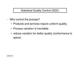
Statistical Process Control (SPC) • Statistical technique used to ensure process is making product to standard. It can also monitor, measure, and correct quality problems. • Control charts are graphs that show upper and lower limits for the process we want to control. Thus, SPC involves taking samples of the process output and plotting the averages on a control chart. 17-6
Statistical Process Control (SPC) (continued) All processes are subject to variability. • Natural causes: Random variations that are uncontrollable and exist in processes that are statistically ‘in control.’ • Assignable causes: Correctable problems that are not random and can be controlled. • Examples: machine wear, unskilled workers, poor material. The objective of control charts is to identify assignable causes and prevent them from reoccurring. 17-7
Statistical Process Control Steps No Produce Good Start Provide Service Assign. Take Sample Causes? Yes Inspect Sample Stop Process Create Find Out Why Control Chart 17-8
Control Chart Patterns Upper control chart limit Target Normal behavior. One point out above. Investigate for cause. One point out below. Investigate for cause. Lower control chart limit 17-9
Control Chart Patterns (continued) Upper control chart limit Target Two points near upper control. Investigate for cause. Two points near lower control. Investigate for cause. Run of 5 points above central line. Investigate for cause. Lower control chart limit 17-10
Control Chart Patterns (continued) Upper control limit Target Erratic behavior. Investigate. Run of 5 points below central line. Investigate for cause. Trends in either Direction. Investigate for cause of progressive change. Lower control limit 17-11
Control Chart Types Continuous Numerical Data Categorical or Discrete Numerical Data Control Charts Variables Attributes Charts Charts R P C X Chart Chart Chart Chart 17-12
Control Charts for Variables - CLT The central limit theorem (CLT) says that the distribution of sample means will follow a normal distribution as the sample size grows large. µ = µ and δ = δ n - - x x x 17-14
Sampling Distribution of Sample Means 99.7% of all x fall within ± 3 x 95.5% of all x fall within ± 2 x 17-15
Control Charts for Variables _ X charts measure the central tendency of a process and indicate whether changes have occurred. R charts values indicate that a gain or loss in uniformity has occurred. X charts and R charts are used together to monitor variables. - 17-16
Steps to Follow in Using X and R Charts __ 1. Collect 20 - 25 samples of n = 4, or n = 5 from a stable process. Compute the mean and range of each sample. 2. Compute the overall means. Set appropriate control limits - usually at 99.7 level. Calculate upper and lower control limits. If process not stable, use desired mean instead of sample mean. 3. Graph the sample means and ranges on their respective control charts. Look to see if any fall outside acceptable limits. 17-17
Steps to Follow in Using X and R Charts (continued) __ 4. Investigate points or patterns that indicate the process is out of control. Try to assign causes for the variation, then resume the process. 5. Collect additional samples. If necessary, re-validate the control limits using the new data. 17-18
Setting Control Limits for the X Chart Control Limits From Table Sample Range at Time i Sample Mean at Time i # of Samples 17-19
Setting Control Limitsfor the R Chart From Table Sample Range at Time i # Samples 17-20
Super Cola Example: x and R Chart Super Cola bottles soft drinks labeled “net weight 16 ounces.” Several batches of 5 bottles each revealed the following: Each batch has 5 bottles of cola _ Construct a X and R chart for the data 17-22
Super Cola Example: x and R Chart Step 1: Collected 20 samples with 5 bottles in each. Compute the mean and range of each batch. The data are given on the previous slide. 17-23
Super Cola Example: x and R Chart Step 2: Compute the overall means and range (x , R), calculate the upper and lower control limits at the 99.7%: Mean = 16.01 ounces Range = 0.25 ounces For X chart UCL = 16.01 + (0.577)(0.25) = 16.154 LCL = 16.01 – (0.577)(0.25) = 15.866 For R Chart UCL = (2.114)(0.25) = .5285 LCL = (0)(0.25) = 0 _ _ 17-24
Super Cola Example: x and R Chart Step 3: Graph the sample means and determine if they fall outside the acceptable limits. 17-25
Super Cola Example: x and R Chart Step 4: Investigate points or patterns that indicate the process is out of control. Are there any points we should investigate?? 17-26
Super Cola Example: x and R Chart Step 5: Collect additional data and revalidate the control limits using the new data.This is particularly important for Super Cola because the original control limits were obtained from ‘unstable’ data. 17-27
Control Charts for Attributes p chartsmeasure the percent defective in a sample and are used to control attributes that typically follow the binomial distribution. c chartsmeasure the count of the number defective and are used to control the number of defects per unit. The Poisson distribution is its basis.For example: • % of mortalities per month versus # of mortalities per month. • % of typed pages with mistakes vs. # of mistakes per page. • % of hamburgers without pickles per shift vs. # of missing pickles per shift. 17-28
Setting Control Limitsforp Chart - p ( 1 p ) = + UCL p z P n - p ( 1 p ) = - UCL p z P n z = 2 for 95.5% limits; z = 3 for 99.7% limits # Defective items in sample i Size of sample i 17-29
ARCO p Chart Example Data entry clerks at ARCO key in thousands of insurance records each day. One hundred records were obtained from 20 clerks and checked for accuracy. p = 0.04 17-30
ARCO p Chart Example (continued) - p ( 1 p ) = + = 0.04 – 3 (.04)(.96) = 0.04 + 3 (.04)(.96) UCL p z P n 100 100 - p ( 1 p ) = - UCL p z P n So, UCL = 0.10 LCL = 0… cannot have a negative percent defective 17-31
ARCO’s pChart Example (continued) UCLp = 0.10 p-Chart .12 .11 .10 .09 Fraction Defective .08 .07 .06 .05 .04 .03 .02 .01 1 2 3 4 5 6 7 8 9 1 0 1 1 1 2 1 3 1 4 1 5 1 6 1 7 1 8 1 9 2 0 .00 LCLp = 0.00 Sample Number What can you say about the accuracy of ARCO’s clerks??? 17-32
Setting Control Limitsforc Chart UCL = c + z cLCL = c – z c z = 2 for 95.5% limits; z = 3 for 99.7% limits Where c = average of all of the samples 17-33
Red Top Cab c Chart Example Red Top Cab Company is interested in studying the number of complaints it receives about the poor cab driver behavior. For nine days the manager recorded the total number of calls he received. c = 6 complaints per day UCL = 6 + 3 ( 6 ) = 13.35 LCL = 6 – 3 ( 6 ) = 0… cannot have negative mistakes. 17-34
Red Top Cab Company c Chart Example (continued) After the control chart was posted prominently, the number of complaints dropped to an average of 3 per day. Can you explain why this may have occurred??? 17-35