Download
1 / 97
970 likes | 1.14k Vues
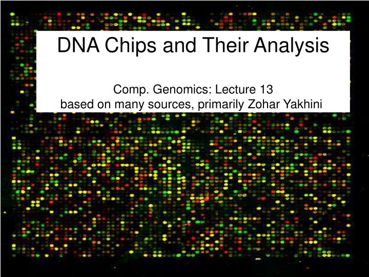
DNA Chips and Their Analysis Comp. Genomics: Lecture 13 based on many sources, primarily Zohar Yakhini. DNA Microarras: Basics. What are they. Types of arrays (cDNA arrays, oligo arrays). What is measured using DNA microarrays. How are the measurements done?.

E N D
DNA Chips and Their AnalysisComp. Genomics: Lecture 13based on many sources, primarily Zohar Yakhini
DNA Microarras: Basics • What are they. • Types of arrays (cDNA arrays, oligo arrays). • What is measured using DNA microarrays. • How are the measurements done?
DNA Microarras: Computational Questions • Design of arrays. • Techniques for analyzing experiments. • Detecting differential expression. • Similar expression: Clustering. • Other analysis techniques (mmmmmany). • Machine learning techniques, and applications for advanced diagnosis.
What is a DNA Microarray (I) • A surface (nylon, glass, or plastic). • Containing hundreds to thousand pixels. • Each pixel has copies of a sequence of single stranded DNA (ssDNA). • Each such sequence is called a probe.
What is a DNA Microarray (II) • An experiment with 500-10k elements. • Way to concurrently explore the function of multiple genes. • A snapshot of the expression level of 500-10k genes under given test conditions
Some Microarray Terminology • Probe: ssDNA printed on the solid substrate (nylon or glass). These are short substrings of the genes we are going to be testing • Target: cDNA which has been labeled and is to be washed over the probe
Back to Basics: Watson and Crick James Watson and Francis Crick discovered, in 1953, the double helix structure of DNA. From Zohar Yakhini
AATGCTTAGTC TTACGAATCAG AATGCGTAGTC TTACGAATCAG Perfect match One-base mismatch Watson-Crick Complimentarity A binds to T C binds to G From Zohar Yakhini
Array Based Hybridization Assays (DNA Chips) • Array of probes • Thousands to millions of differentprobe sequences per array. Unknown sequence or mixture (target).Many copies. From Zohar Yakhini
Array Based Hyb Assays • Target hybs to WC complimentary probes only • Therefore – the fluorescence pattern is indicative of the target sequence. From Zohar Yakhini
DNA Sequencing Sanger Method • Generate all A,C,G,T – terminated prefixes of the sequence, by a polymerase reaction with terminating corresponding bases. • Run in four different gel lanes. • Reconstruct sequence from the information on the lengths of all A,C,G,T – terminated prefixes. • The need for 4 different reactions is avoided by using differentially dye labeled terminating bases. From Zohar Yakhini
Transcription Translation mRNA Protein Central Dogma of Molecular Biology(reminder) Cells express different subset of the genes in different tissues and under different conditions Gene (DNA) From Zohar Yakhini
Expression Profiling on MicroArrays • Differentially label the query sample and the control (1-3). • Mix and hybridize to an array. • Analyze the image to obtain expression levels information. From Zohar Yakhini
Microarray: 2 Types of Fabrication • cDNA Arrays: Deposition of DNA fragments • Deposition of PCR-amplified cDNA clones • Printing of already synthesized oligonucleotieds • Oligo Arrays: In Situ synthesis • Photolithography • Ink Jet Printing • Electrochemical Synthesis By Steve Hookway lecture and Sorin Draghici’s book “Data Analysis Tools for DNA Microarrays”
cDNA Microarrays vs. Oligonucleotide Probes and Cost By Steve Hookway lecture and Sorin Draghici’s book “Data Analysis Tools for DNA Microarrays”
Photolithography (Affymetrix) • Similar to process used to generate VLSI circuits • Photolithographic masks are used to add each base • If base is present, there will be a “hole” in the corresponding mask • Can create high density arrays, but sequence length is limited Photodeprotection mask C From “Data Analysis Tools for DNA Microarrays” by Sorin Draghici
Photolithography (Affymetrix) From Zohar Yakhini
Ink Jet Printing • Four cartridges are loaded with the four nucleotides: A, G, C,T • As the printer head moves across the array, the nucleotides are deposited in pixels where they are needed. • This way (many copies of) a 20-60 base long oligo is deposited in each pixel. By Steve Hookway lecture and Sorin Draghici’s book “Data Analysis Tools for DNA Microarrays”
C T A G Ink Jet Printing (Agilent) The array is a stack of images in the colors A, C, G, T. … From Zohar Yakhini
Inkjet Printed Microarrays Inkjet head, squirting phosphor-ammodites From Zohar Yakhini
Electrochemical Synthesis • Electrodes are embedded in the substrate to manage individual reaction sites • Electrodes are activated in necessary positions in a predetermined sequence that allows the sequences to be constructed base by base • Solutions containing specific bases are washed over the substrate while the electrodes are activated From “Data Analysis Tools for DNA Microarrays” by Sorin Draghici
Preparation of Samples • Use oligo(dT) on a separation column to extract mRNA from total cell populations. • Use olig(dT) initiated polymerase to reverse transcribe RNA into fluorescence labeled cDNA. RNA is unstable because of environment RNA-digesting enzymes. • Alternatively – use random priming for this purpose, generating a population of transcript subsequences From Zohar Yakhini
Expression Profiling on MicroArrays • Differentially label the query sample and the control (1-3). • Mix and hybridize to an array. • Analyze the image to obtain expression levels information. From Zohar Yakhini
Expression Profiling: a FLASH Demo URL: http://www.bio.davidson.edu/courses/genomics/chip/chip.html
Expression Profiling – Probe Design Issues • Probe specificity and sensitivity. • Special designs for splice variations or other custom purposes. • Flat thermodynamics. • Generic and universal systems From Zohar Yakhini
Hybridization Probes • Sensitivity:Strong interaction between the probe and its intended target, under the assay's conditions.How much target is needed for the reaction to be detectable or quantifiable? • Specificity:No potential cross hybridization. From Zohar Yakhini
Specificity • Symbolic specificity • Statistical protection in the unknown part of the genome. Methods, software and application in collaboration with Peter Webb, Doron Lipson. From Zohar Yakhini
Reading Results: Color Coding • Numeric tables are difficult to read • Data is presented with a color scale • Coding scheme: • Green = repressed (less mRNA) gene in experiment • Red = induced (more mRNA) gene in experiment • Black = no change (1:1 ratio) • Or • Green = control condition (e.g. aerobic) • Red = experimental condition (e.g. anaerobic) • We usually use ratio Campbell & Heyer, 2003
Thermal Ink Jet Arrays, by Agilent Technologies In-Situ synthesized oligonucleotide array. 25-60 mers. cDNA array, Inkjet deposition
Application of Microarrays • We only know the function of about 30% of the 30,000 genes in the Human Genome • Gene exploration • Functional Genomics • First among many high throughput genomic devices http://www.gene-chips.com/sample1.html By Steve Hookway lecture and Sorin Draghici’s book “Data Analysis Tools for DNA Microarrays”
A Data Mining Problem • On a given microarray, we test on the order of 10k elements in one time • Number of microarrays used in typical experiment is no more than 100. • Insufficient sampling. • Data is obtained faster than it can be processed. • High noise. • Algorithmic approaches to work through this large data set and make sense of the data are desired.
Informative Genes in aTwo Classes Experiment • Differentially expressed in the two classes. • Identifying (statistically significant) informative genes • - Provides biological insight • - Indicate promising research directions • - Reduce data dimensionality • - Diagnostic assay From Zohar Yakhini
Informative genes+ + + + + + + + - - - - - - -- - - - - - -+ + + + + + + + - - - - + - -+ + - + + + + + etc Non-informative genes + - + - + + + + - - + + - - -- + + - + - -+ + - + + - - + + - - - + + -+ + - + + - + - etc Scoring Genes Expression pattern and pathological diagnosis information (annotation), for a single gene + + - - + + + - - + - - + + - a1 a2 a3 a4 a5 a6 a7 a8 a9 a10 a11 a12 a13 a14 a15 Permute the annotation by sorting the expression pattern (ascending, say). From Zohar Yakhini
6 7 # of errors = min(7,8) = 7. Ex 2: A perfect single gene classifier gets a score of 0. + + + + + + + + - - - - - - - 0 Threshold Error Rate (TNoM) Score Find the threshold that best separates tumors from normals, count the number of errors committed there. Ex 1: - + + - + - -+ + - + + - - + From Zohar Yakhini
p-Values • Relevance scores are more useful when we can compute their significance: • p-value: The probability of finding a gene with a given score if the labeling is random • p-Values allow for higher level statistical assessment of data quality. • p-Values provide a uniform platform for comparing relevance, across data sets. • p-Values enable class discovery From Zohar Yakhini
BRCA1 Differential Expression Genes over-expressed in BRCA1 wildtype Genes over-expressed in BRCA1 mutants Collab with NIH NEJM 2001 Sporadic sample s14321 With BRCA1-mutant expression profile BRCA1 mutants BRCA1 Wildtype From Zohar Yakhini
Small, efficient diagnostic assays Perform this using different choices of genes subsets sizes Data Analysis: Leave One Out Cross Validation (LOOCV) • Repeat, for each tissue (tumor/normal) • “Hide” the label of the test tissue • Diagnose the test tissue based on the remaining data • Compare the diagnosis to the hidden label From Zohar Yakhini
95% success rate (21/22) • Sporadic tissue (14321) consistently classified as BRCA1 • BRCA1 gene is normal, but silenced in the patient’s DNA BRCA1 LOOCV Results From Zohar Yakhini
Lung Cancer Informative Genes Data from Naftali Kaminski’s lab, at Sheba. • 24 tumors (various types and origins) • 10 normals (normal edges and normal lung pools) From Zohar Yakhini
And Now: Global Analysisof Gene Expression Data First (but not least): Clustering either of genes, or of experiments
Example data: fold change (ratios) What is the pattern? Campbell & Heyer, 2003
Example data 2 Campbell & Heyer, 2003
Pearson Correlation Coefficient, r.values in [-1,1] interval • Gene expression over d experiments is a vector in Rd, e.g. for gene C: (0, 3, 3.58, 4, 3.58, 3) • Given two vectors X and Y that contain N elements, we calculate r as follows: Cho & Won, 2003
Example: Pearson Correlation Coefficient, r • X = Gene C = (0, 3.00, 3.58, 4, 3.58, 3)Y = Gene D = (0, 1.58, 2.00, 2, 1.58, 1) • ∑XY = (0)(0)+(3)(1.58)+(3.58)(2)+(4)(2)+(3.58)(1.58)+(3)(1) = 28.5564 • ∑X = 3+3.58+4+3.58+3 = 17.16 • ∑X2 = 32+3.582+42+3.582+32 = 59.6328 • ∑Y = 1.58+2+2+1.58+1 = 8.16 • ∑Y2 = 1.582+22+22+1.582+12 = 13.9928 • N = 6 • ∑XY – ∑X∑Y/N = 28.5564 – (17.16)(8.16)/6 = 5.2188 • ∑X2 – (∑X)2/N = 59.6328 – (17.16)2/6 = 10.5552 • ∑Y2 – (∑Y)2/N = 13.9928 – (8.16)2/6 = 2.8952 • r = 5.2188 / sqrt((10.5552)(2.8952)) = 0.944
Example data: Pearson correlation coefficients Campbell & Heyer, 2003
Example: Reorganization of data Campbell & Heyer, 2003
Spearman Rank Order Coefficient • Replace each entry xi by its rank in vector x. • Then compute Pearson correlation coefficients of rank vectors. • Example: X = Gene C = (0, 3.00, 3.41, 4, 3.58, 3.01) Y = Gene D = (0, 1.51, 2.00, 2.32, 1.58, 1) • Ranks(X)= (1,2,4,6,5,3) • Ranks(Y)= (1,3,5,6,4,2) • Ties should be taken care of: (1) rare (2) randomize (small effect)
Grouping and Reduction • Grouping: Partition items into groups. Items in same group should be similar. Items in different groups should be dissimilar. • Grouping may help discover patterns in the data. • Reduction: reduce the complexity of data by removing redundant probes (genes).
Unsupervised Grouping: Clustering • Pattern discovery via clustering similarly expressed genes together • Techniques most often used: • k-Means Clustering • Hierarchical Clustering • Biclustering • Alternative Methods: Self Organizing Maps (SOMS), plaid models, singular value decomposition (SVD), order preserving submatrices (OPSM),……
Clustering Overview • Different similarity measures in use: • Pearson Correlation Coefficient • Cosine Coefficient • Euclidean Distance • Information Gain • Mutual Information • Signal to noise ratio • Simple Matching for Nominal