Download
1 / 12
120 likes | 214 Vues
A map f : R n R defined by f ( x 1 ,x 2 ,…, x n ) is called a scalar field. A map F : R 2 R 2 defined by F ( x,y ) = ( F 1 ( x,y ) , F 2 ( x,y ) ) is called a vector field in the plane.

E N D
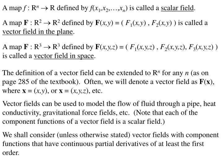
A map f : Rn R defined by f(x1,x2,…,xn) is called a scalar field. A map F : R2 R2 defined by F(x,y) = ( F1(x,y) , F2(x,y) ) is called a vector field in the plane. A map F : R3 R3 defined by F(x,y,z) = ( F1(x,y,z) , F2(x,y,z), F3(x,y,z) ) is called a vector field in space. The definition of a vector field can be extended to Rn for any n (as on page 285 of the textbook). Often, we will denote a vector field as F(x), where x = (x,y), or x = (x,y,z), etc. Vector fields can be used to model the flow of fluid through a pipe, heat conductivity, gravitational force fields, etc. (Note that each of the component functions of a vector field is a scalar field.) We shall consider (unless otherwise stated) vector fields with component functions that have continuous partial derivatives of at least the first order.
Sketch the vector field V(x,y) = (– y , x ) = – yi + xj . V(1,0) = (0,1) Work Area Sketch
Sketch the vector field V(x,y) = (– y , x ) = – yi + xj . V(1,0) = (0,1) V(1,1) = (–1,1) Work Area Sketch
Sketch the vector field V(x,y) = (– y , x ) = – yi + xj . V(1,0) = (0,1) V(1,1) = (–1,1) V(0,1) = (–1,0) Work Area Sketch
Sketch the vector field V(x,y) = (– y , x ) = – yi + xj . V(1,0) = (0,1) V(1,1) = (–1,1) V(0,1) = (–1,0) V(–1,1) = (–1,–1) Work Area Sketch
Sketch the vector field V(x,y) = (– y , x ) = – yi + xj . V(1,0) = (0,1) V(1,1) = (–1,1) V(0,1) = (–1,0) V(–1,1) = (–1,–1) V(–1,0) = (0,–1) Work Area Sketch
Sketch the vector field V(x,y) = (– y , x ) = – yi + xj . V(1,0) = (0,1) V(1,1) = (–1,1) V(0,1) = (–1,0) V(–1,1) = (–1,–1) V(–1,0) = (0,–1) V(–1,–1) = (1,–1) V(0,–1) = (1,0) V(1,–1) = (1,1) Work Area Sketch Continue with the sketch. Compare with Figure 4.3.3 on page 286.
y – x ——— , ——— x2 + y2 x2 + y2 yi – xj ——— . x2 + y2 Sketch the vector field V(x,y) = ( ) = V(1,0) = (0, –1) V(0,1) = (1,0) V(–1,0) = (0,1) V(0,–1) = (–1,0) V(2,0) = (0,–1/2) V(0,2) = (1/2,0) V(–2,0) = (0,1/2) V(0,–2) = (–1/2,0) Compare with Figure 4.3.4 on page 287.
A vector field F(x) is a gradient vector field, if we can find a function f(x) such that f(x) = F(x) . Determine whether or not the vector field F(x,y) = ( x / x2 + y2 , y / x2 + y2 ) is a gradient vector field. In order for F(x,y) = (x / x2 + y2 , y / x2 + y2 ) to be a gradient, we must find f(x,y) so that fx(x,y) = and fy(x,y) = x / x2 + y2y / x2 + y2 . If this were possible, then it must be true that fxy(x,y) = fyx(x,y). It is easy to verify that fxy(x,y) = fyx(x,y) = – xy / (x2 + y2)3/2 . Consequently, F(x,y) = is a gradient vector field. To actually find f(x,y), we observe that f(x,y) = and f(x,y) = ( x / x2 + y2 , y / x2 + y2 ) (x2 + y2)1/2 + k1(y) (x2 + y2)1/2 + k2(x) . Then, we must have that f(x,y) = (x2 + y2)1/2 + k .
Determine whether or not the vector field V(x,y) = ( y , – x ) is a gradient vector field. In order for V(x,y) = ( y , – x ) to be a gradient, we must find f(x,y) so that fx(x,y) = and fy(x,y) = . y – x If this were possible, then it must be true that fxy(x,y) = fyx(x,y). It is easy to verify that fxy(x,y) = and fyx(x,y) = 1 – 1 . Consequently, V(x,y) = ( y , – x ) is not a gradient vector field.
If F is a vector field, then a flow line for F is a path c(t) such that c(t) = F(c(t)) , that is, F yields the velocity field of the path c(t). Consider the vector field F(x,y) = – yi + xj . (a) Is c1(t) = (10cos t , 10sin t) = (10cos t)i + (10sin t)j a flow line of F ? (b) Is c2(t) = (10cos(2– t) , 10sin(2 –t)) = (10cos(2 –t))i + (10sin(2 –t))j a flow line of F ? c1(t) = – (10sin t)i + (10cos t)j F(c1(t)) = – (10sin t)i + (10cos t)j Consequently, c1(t) = (10cos t)i + (10sin t)j is a flow line of the vector field F . c2(t) = (10sin(2 –t))i– (10cos(2 –t))j F(c2(t)) = (–10sin(2 –t))i+ (10cos(2 –t))j Consequently, c2(t) = (10cos(2 –t))i + (10sin(2 –t))j is not a flow line of the vector field F .
(c) Is c3(t) = (et, e–t) = eti + e–tj a flow line of F ? c3(t) = eti–e–tj F(c3(t)) = – e–ti+etj Consequently, c3(t) = eti + e–tj is not a flow line of the vector field F . (d) What other flow lines of the vector field F(x,y) can be found? In order for c(t) = x(t)i + y(t)j to be a flow line, we must have c(t) = F(c(t)), that is, x (t)i + y (t)j = – y(t)i + x(t)j . Solutions to such problems can be suggested by examining a picture of the vector field (or solutions can be found by solving the corresponding system of differential equations). Paths of the form c(t) = ( r0cos(t + t0) , r0sin(t + t0) ) will work for any constants r0 and t0.