Particle Identification

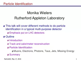
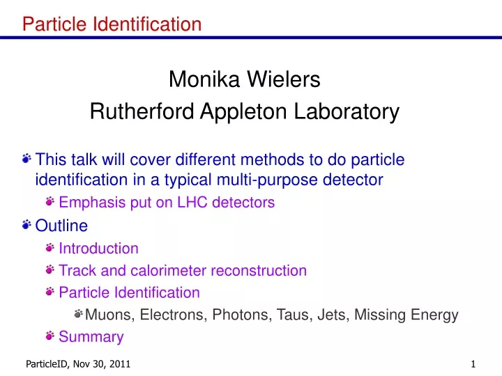
Particle Identification • This talk will cover different methods to do particle identification in a typical multi-purpose detector • Emphasis put on LHC detectors • Outline • Introduction • Track and calorimeter reconstruction • Particle Identification • Muons, Electrons, Photons, Taus, Jets, Missing Energy • Summary Monika Wielers Rutherford Appleton Laboratory

Collision: What happens? • During collisions of e.g. 2 particles energy is used to create new particles • Particles produced are non stable and will decay in other (lighter) particles • Cascade of particles is produced • Therefore • We cannot “see” the reaction itself • To reconstruct the process and the particle properties, need maximum information about end-products

Introduction • These end-product are the basic input to any physics analysis • E.g. if you want to reconstruct a Z boson, you need to look for events with 2 muons, electrons or jets and then calculate the invariant mass • There will be events in which you also find 2 objects and which have a similar invariant mass • Better do your particle identification right, so that you have to deal with little background q e+ Z0 e- q

Global Detector Systems Overall Design Depends on: • Number of particles • Event topology • Momentum/energy • Particle type  No single detector does it all…  Create detector systems Fixed Target Geometry Collider Geometry • Limited solid angle (d coverage (forward) • Easy access (cables, maintenance) • “full” solid angle d coverage • Very restricted access

How to detect particles in a detector • Tracking detector • Measure charge and momentum of charged particles in magnetic field • Electro-magnetic calorimeter • Measure energy of electrons, positrons and photons • Hadronic calorimeter • Measure energy of hadrons (particles containing quarks), such as protons, neutrons, pions, etc. Neutrinos are only detected indirectly via ‘missing energy’ not recorded in the calorimeters • Muon detector • Measure charge and momentum of muons

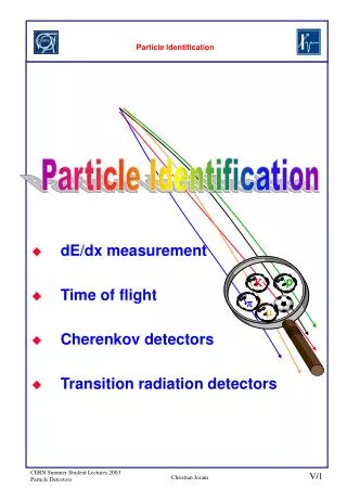
How to detect particles in a detector • Use the inner tracking detector, the calorimeters and the muon detector information • There can be also some special detectors to identify particles • /K/p identification using Cerenkov effect (Sajan‘s talk) • Dedicated photon detector (Sajan‘s talk) • There are other things which I won‘t explain • Energy loss measurement in tracking detector for /K/p separation (dE/dx) • Transition radiation detectors for e/ separation • ...

ATLAS and CMS Detectors Revisited ATLAS • Two different approaches for detectors CMS

Why do we need to reconstruct all of this... • ... To measure the particles and decays produced in the collisions • Deduce from which physics process they come

Detector Reconstruction • Tracking • Calorimetry

As these terms will crop up during the talk... Coordinate system used in hadron collider experiments • Particle can be described as • p =(px, py, pz) • In hadron collider we use • p, ,  •  is called “pseudo-rapidity“ • Angle between particle momentum and beam axis (z-direction) • Good quantity as number of particles per  unit is constant •  is angle in x-y-plane • px = pTcos(), py = pTsin(), pT=px2+py2

Tracking: Role of the inner detector • Extrapolate back to the point of origin. Reconstruct: • Measure the trajectory of charged particles • Fit curve to several measured points (“hits”) along the track. • measure the momentum of charged particles from their curvature in a magnetic field • Primary vertices • reconstruct primary vertex and thus identify the vertex associated with the interesting “hard” interaction • Secondary vertices • Identify tracks from tau-leptons, b and c-hadrons, which decay inside the beam pipe, by lifetime tagging • Reconstruct strange hadrons, which decay in the detector volume • Identify photon conversions • More on tracking detectors in Guilio’s talk next year

Track reconstruction • 1D straight line fit as simple case • Two perfect measurements in 2 layers of the detector • no measurement uncertainty • just draw a straight line through them and extrapolate • Imperfect measurements give less precise results • the farther you extrapolate, the less you know • Smaller errors and more points help to constrain the possibilities. • But how to find the best point from a large set of points? • Parameterise track (helix is you have magnetic field) • Find track parameters by Least-Squares-Minimisation • Gives you errors , d predicted track position at ith hit position of ith hit uncertainty of ith measurement

Track Reconstruction • Reality is a bit more complicated • Particles interact with matter • energy loss • change in direction • This is multiple scattering • Your track parameterisation needs to take this into account • Do calculate very precisely would take too long, therefore, work outward N times

Track Reconstruction • Reality is a bit more complicated • Particles interact with matter • energy loss • change in direction • This is multiple scattering • Your track parameterisation needs to take this into account • Do calculate very precisely would take too long, therefore, work inward N times • In each step extrapolate to next layer, using info from current track parameters, expected scattering error, and measurement in next layer • Needs starting estimate (seed) and may need some iterations, smoothing

Track Reconstruction • Reality is a bit more complicated • Particles interact with matter • energy loss • change in direction • This is multiple scattering • Your track parameterisation needs to take this into account • Do calculate very precisely would take too long, therefore, work inward N times • In each step extrapolate to next layer, using info from current track parameters, expected scattering error, and measurement in next layer • Needs starting estimate (seed) and may need some iterations, smoothing • This method is based on theory of the Kalman Filter

B-tagging • b hadrons are • long-lived (c~450 μm) • Massive • Signature: displaced vertex • Important parameters are • d0 = impact parameter (point closest approach in the x-yplane) • Lxy = distance between primary and secondary vertices • As LHC is a b- (and even top) factory, b-tagging is a very useful measure Primary Secondary Tertiary vertex

Concept of Calorimetry • Particle interaction in matter (depends on the impinging particle and on the kind of material) • Destructive interaction • Energy loss transfer to detectable signal (depends on the material) • Signal collection (depends on signal, many techniques of collection) • Electric: charge collection • Optic : light collection • Thermal : temperature ionisation scintillation SE Cerenkov

Calorimeter • Calorimeters have been introduced mainly to measure the total energy of particles • Versatile detectors, can measure also position, angle, timing for charged & neutral particles (even neutrinos through missing (transverse) energy (if hermetic)) • Compact detectors: shower length increase only logarithmically with E • Unlike tracking detectors, E resolution improves with increasing E • Divide into categories: electro-magnetic (EM) calorimeters and hadron calorimeters • Typically subdivided into several layers and many readout units (cells) • More on calorimetry in Dave’s talk

Cluster Reconstruction • Clusters of energy in a calorimeter are due to the original particles • Clustering algorithm groups individual channel energies • Don’t want to miss any, don’t want to pick up fakes • Ways to do clustering • Just scan the calorimeter cell energies and look for higher energetic cells which give local maximum, build cluster around • Can used fixed “window” size or can do it dynamically and add cell if above a given threshold

Particle Identification • Muon • Electron and Photon • Taus • Jets • Missing transverse energy

Muon Identification • Because of it’s long lifetime, the muon is basically a stable particle for us (c ~ 700 m) • It does not feel the strong interaction • Therefore, they are very penetrating • Obviously very similar to inner detector tracking • But much less combinatorics to deal with • Reconstruct tracks in muon and inner detector and combine them • Strategy • Find tracks in the muon system • Match with track in inner tracker • Combine track measurements • Consistent with MIP • Little or no energy in calorimeters • Very clean signal!

Another Complication: Pileup • When the LHC collides bunches of protons we can get more than one p-p interaction – this is called pileup • These are mainly soft interactions producing low momentum particles • The number of pileup interactions depends on the LHC parameters • How many protons per bunch • How small the bunches • At design luminosity of 1034 cm-2s-1 we expect ~25 overlapping p-p collisions, in 2011 we already had up to around 20) • We can usually identify which tracks are from which interactions by combining tracks that come from the same vertex

Z in pile-up environment • Z event with 11 reconstructed vertices. • Tracks with transverse momentum above 0.5 GeV are shown (pT>0.5GeV).

Z in pile-up environment • Z event with 11 reconstructed vertices. • Looks already much better if we increase the pT cut to 2 GeV

Z in pile-up environment • Z event with 11 reconstructed vertices. • Even better if we increase the pT cut to 10 GeV

Electrons and Photons • Energy deposit in EM calorimeter • Energy nearly completely deposited in EM calorimeter • Little or no energy in had calorimeter (hadronic leakage) • “Narrow“ cluster or shower shape in EM calorimeter • Electrons has a track pointing to the cluster • If there is no track: photon • But be careful, photons can convert before reaching the calorimeter • Final Electron momentum measurement can come from tracking or calorimeter information (or a combination of both) • Often want isolated electrons • Require little calorimeter energy or tracks in the region near the electron

Electron and photon identification Transverse shower shape in 2nd EM layer (ATLAS) Electron or photon cut jet • Leakage into 1st layer of hadronic calorimeter • Analyse shape of the cluster in the different layers of the EM calo • “narrow“ e/ shape vs “broad“ one from mainly jets • Look for sub-structures • Preshower in CMS, 1st EM layer with very fine granularity in ATLAS • Very useful for 0 /  separation, 2 photons from 0 tend to end up in the same cluster at LHC energies • Look at how well your track position matches with the one from the calorimeter • Use E/p ATLAS

Electron and photon identification • As shower shape from jets broader it should be easy to separate electrons/photons from jets • However have many thousands more jets than electrons, so need the rate of jets faking an electron to be very small ~10-4 for electrons and several times 10-3 for photons • Need complex identification algorithms to give the rejection whilst keeping a high efficiency

Bremsstrahlung • Electrons can emit photons in the presence of material • We have a bit more that we wanted in ATLAS and CMS and there is high chance this happens • Track has „kink“ • At LHC energies: • electron and photon (typically) end up in the same cluster • Electron momentum is reduced • E/p distribution will show large tails • Methods for bremsstrahlung recovery • Gaussian Sum Filter, Dynamic Noise Adjustment • Use of calorimeter position to correct for bremsstrahlung • Kink reconstruction, use track measurement before kink

Conversion reconstruction • Photons can produce electron pairs in the presence of material • Find 2 tracks in the inner detector from the same secondary vertex • Need for outside-in tracking • However, can be useful: • Can use conversions to x-ray detector and determine material before calorimeter (i.e. tracker) ATLAS CDF

Taus • Decays • 17% in muons • 17% in electrons • ~65% of ’s decay hadronically in 1- or 3-prongs (, +n0 or 3, 3+n0) • For reconstruct hadronic taus • Look for “narrow“ jets in calorimeter (EM + hadronic) • i.e. measure EM and hadronic radius (measurement of shower size in -): EcellR2cell/Ecell • Form ΔR cones around tracks • tau cone • isolation cone • associate tracks (1 or 3)

Jets • In “nature” do not observe quarks and gluons directly, only hadrons, which appear collimated into jets • Jet definition (experimental point of view): bunch of particles generated by hadronisation of a common otherwise confined source • Quark-, gluon fragmentation • Signature • energy deposit in EM and hadronic calorimeters • Several tracks in the tracker

Jet Reconstruction • How to reconstruct the jet? • Group together the particles from hadronisation • 2 main types • Cone • kT

Infrared safety Adding or removing soft particles should not change the result of jet clustering Collinear safety Splitting of large pT particle into two collinear particles should not affect the jet finding Invariance under boost Same jets in lab frame of reference as in collision frame Order independence Same jet from partons, particles, detector signals Many jet algorithms don’t fulfill above requirements! Theoretical requirement to jet algorithm choices collinear sensitivity (1) (signal split into two towers below threshold) infrared sensitivity (artificial split in absence of soft gluon radiation) collinear sensitivity (2) (sensitive to Et ordering of seeds)

Types of jet reconstruction algorithms: cone Example: iterative cone algorithms • Find particle with largest pT above a seed threshold • Draw a cone of fixed size around this particle • . • Collect all other particles in cone and recalculate cone directions • Take next particle from list if above pT seed threshold • Repeat procedure and find next jet candidate • Continue until no more jet above threshold can be reconstructed • Check for overlaps between jets • Add lower pT jet to higher pT jet if sum of particle pT in overlap is above a certain fraction of the lower pT jet (merge) • Else remove overlapping particles from higher pT jet and add to lower pT jet (split) • All surviving jet candidates are the final jets • Different varieties: (iterative) fixed cone, seedless cone, midpoint…

Types of jet reconstruction algo.: Recursive Recombination • Motivated by gluon splitting function • Classic procedure • Calculate all distances dji for list of particles / cell energies / jet candidates • . with , n=1 • Find smallest dij, if lower than cutoff combine (combine particles if relative pT < pT of more energetic particle) • Remove i and j from list • Recalculate all distances, continue until all particles are removed or called a jet • Alternatives • Cambridge / Aachen (n=0) • Uses angular distances only • Anti-kT (n= -1, preferred by ATLAS/CMS) • First cluster high E with high E and high E with low E particles This keeps jets nicely round

Energy Flow • You might want to combine tracking with calorimeter information • Lot‘s of info given in Dave‘s talk • Use “best measurement” of each component • Charged tracks = Tracker • e/photons = Electromagnetic calorimeter • Neutral hadrons from hadronic calo: only 10% • Critical points: • Very fine granularity • Confusion due to shower overlaps in calorimeter • Very large number of channels • Successfully used for ALEPH experiment and now by CMS experiment (in both case rather poor HCAL )

Missing Transverse Energy • Missing energy is not a good quantity in a hadron collider as much energy from the proton remnants are lost near the beampipe • Missing transverse energy (ETmiss) much better quantity • Measure of the loss of energy due to neutrinos • Definition: • . • Best missing ET reconstruction • Use all calorimeter cells which are from a clusters from electron, photon, tau or jet • Use all other calorimeter cells • Use all reconstructed particles not fully reconstructed in the calorimeter • e.g. muons from the muon spectrometer

Missing Transverse Energy • But it‘s not that easy... • Electronic noise might bias your ET measurement • Particles might have ended in cracks / insensitive regions • Dead calorimeter cells • Corrections needed to calorimeter missing ET • Correction for muons • Recall: muons are MIPs • Correct for known leakage effects (cracks etc) • Particle type dependent corrections • Each cell contributes to missing ET according to the final calibration of the reconstructed object (e, , , jet…) • Pile-up effects will need to be corrected for

Missing Transverse Energy • Difficult to understand quantity

Summary • Tried to summarise basic features of particle identification • Muon, Electron, Photon, Tau, Jet, Missing ET • Hope this has been useful as you will need to to use all the reconstructed quantities for any physics analysis

Backup

Gas/Wire Drift Chambers • Wires in a volume filled with a gas (such as Argon/Ethan) • Measure where a charged particle has crossed • charged particle ionizes the gas. • electrical potentials applied to the wires so electrons drift to the sense wire • electronics measures the charge of the signal and when it appears. • To reconstruct the particles track several chamber planes are needed • Example: • CDF COT: 30 k wires, 180 μm hit resolution • Advantage: • low thickness (fraction of X0) • traditionally preferred technology for large volume detectors

Muon Chambers • Purpose: measure momentum / charge of muons • Recall that the muon signature is extraordinarily penetrating • Muon chambers are the outermost layer • Measurements are made combined with inner tracker • Muon chambers in LHC experiments: • Series of tracking chambers for precise measurements • RPC’s: Resistive Plate Chambers • DT’s: Drift Tubes • CSC’s: Cathode Strip Chambers • TGC’s: Thin Gap Chambers Cosmic muon in MDT/RPC

Cluster reconstruction Losses between PS and S1 strips Middle Back e with energy E Longitudinal Leakage Upstream Losses Upstream Material Presampler LAr Calorimeter • Input to clustering: • Cells calibrated at the EM scale • Sum energy in EM calo, correct for losses in upstream material, longitudinal leakage and possible other lossses between calo layers (if applicable) • e.g. • Typically need to find best compromise between best resolution and best linearity

Calorimeters: Hadronic Showers • Much more complex than EM showers • visible EM O(50%) • e, , o • visible non-EM O(25%) • ionization of , p,  • invisible O(25%) • nuclear break-up • nuclear excitation • escaped O(2%) • Only part of the visible energy is measured (e.g. some energy lost in absorber in sampling calorimeter) • calibration tries to correct for it

Useful things to know in the LHC environment

Particle Identification