M. Vellante 1 , M. Piersanti 1 , B. Heilig 2

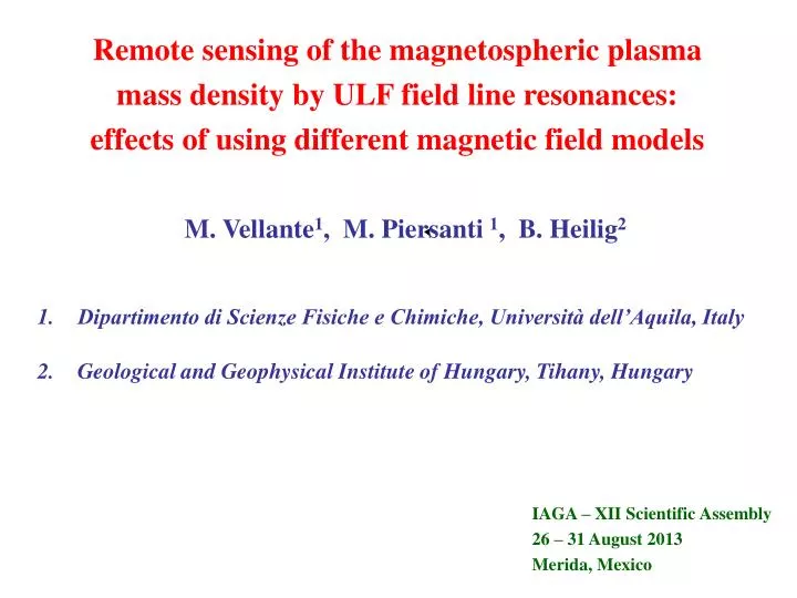
1. Remote sensing of the magnetospheric plasma mass density by ULF field line resonances: effects of using different magnetic field models M. Vellante1, M. Piersanti 1, B. Heilig2 • Dipartimento di Scienze Fisiche e Chimiche, Università dell’Aquila, Italy • Geological and Geophysical Institute of Hungary, Tihany, Hungary IAGA – XII Scientific Assembly 26 – 31 August 2013 Merida, Mexico

2. Inference of the plasma mass density from field line eigenfrequencies Standard procedure for low and middle latitudes: Observed FLR frequencies (fR) correspond to the axisymmetric toroidal mode eigenfrequencies in a dipole field. Assumption: E: wave electric field z = cos (θ), θ: colatitude ρ : mass density along the field line ρo: equatorial mass density Governing equation: d2E/dz2 + λ (1- z2)6ρ(z)/ρo E = 0 • Eigenvalues λare found imposing: • the boundary condition: E = 0 at the altitude (100-200 km) where the wave is reflected • A given functional form for the mass density along the field line. • Common assumption: ρ(r)/ρo = (r / ro) - m For any given L- shell and m value, the inferred equatorial mass density is:

3. IGRF line crossing equator at 2 RE, geomag. long. 80° Dipole line traced from the equatorial point

4. IGRF line crossing equator at 2 RE, geomag. long. 80° Dipole line traced from the equatorial point

7. Dipole field : wave electric field z = cos (), : colatitude RE: Earth radii Arbitrary field geometry (Singer et al., 1981) s distance along the field line B (s) magnetic field ’ (s) =  (s) / h (s)  (s) field line displacement h (s) distance to an adjacent field line

8. Comparison of eq estimates obtained using dipole and IGRF models for possible station pairs of EMMA/SANSA arrays

9. Full longitudinal range analysis

10. Effective equatorial dipole field

11. Effective magnetic dipole moment

12. At high latitudes, and even at middle latitudes during particular conditions, need to consider geomagnetic field geometry more realistic than dipole or IGRF geometry (i.e. Tsyganenko models).

13. T01 model (Tsyganenko 2002a, 2002b) • Input parameters: • Universal Time: to determine the proper coefficients of the internal field (IGRF) and the tilt angle; • Solar wind dynamic pressure; • Dst index; • IMF By and Bz components; • G1, G2: take into account the prehistory state of the magnetosphere (determined by By, Bz, Vsw of the previous hour).

14. For the comparison of inferred densities we assume: eq = eq,0  10B(LL0) 0.3 ≤B≤ 0.9

15. Average solar wind/magnetospheric conditions Low equat. gradient: B = 0.3 High equat. gradient: B = 0.9 eq= eq,0  10B(LL0)

16. Disturbed magnetospheric conditions, Dst = -100

17. MATLAB code determining the equatorial plasma mass density • Input parameters: • observed fundamental eigenfrequency (obtained from FLRID for a given station pair; • geographical coordinates of the middle point of the station pair; • index m of the assumed power-law dependence of the mass density; • Input parameters of the T01 model. • Output parameters: • geomagnetic coordinates of the magnetic equatorial point of the field line (radial distance and longitude) determined by the T01 model; • inferred plasma mass density in that point. • Additional information (apex location, magnetic field at the equatorial point and at the apex, field line length, coordinates of the conjugate point, etc.) are also available.

18. Real-time run • Run every 15 min using: • quasi real-time values of field line eigenfrequencies of all available station pairs (as computed by FLRID); • solar wind and Dst parameters. Real time solar wind data taken from the NOAA Space Weather Prediction Center which provides the latest 2 hours of magnetic and plasma data of the ACE satellite located at the L1 libration point. (http://www.swpc.noaa.gov/ftpdir/lists/ace/ace_mag_1m.txt; http://www.swpc.noaa.gov/ftpdir/lists/ace/ace_swepam_1m.txt) Time-shift to take into account the propagation time of the solar wind from the satellite position to the Earth (typically about 1 hour). Propagated data are resampled at fixed times and hourly running averages (time step 15 min) are produced. Real-time Dst data are taken from the World Data Center for Geomagnetism (Kyoto) http://wdc.kugi.kyoto-u.ac.jp/dst_realtime/

19. To be done: • evaluation of uncertainties associated to the density estimates; • optimization of the implementation of the T01 model in order to decrease the computing time and/or to use a more recent version TS05 which is more reliable for geomagnetic storm events. • examination of other kinds of field-aligned density distributions for low L ? • consideration of more general ionospheric boundary conditions ?

20. Poulter et al., 1988

21. Ozeke and Mann, 2005 The "fixed end" fundamental frequency decreases with decreasing ionospheric Pedersen conductivity.

22. Another possibility is the formation of a quarter wave mode – asymmetric conductivity Allan, 1983 Obana et al. (2008)

23. Acknowledgments The research leading to these results has received funding from the European Union Seventh Framework Programme [FP7/2007-2013] under grant agreement n°263218.

24. Density inference for low L-shells Ionosphere-Plasmasphere Model (M. Förster, GFZ, Potsdam) Physical-numerical model to describe the thermal plasma behaviour in corotating flux tubes conjoining the ionosphere and the plasmasphere. Constituents: O+, H+, He+, O2+, N2+, NO+ Configuration: tilted geomagnetic dipole from 120 km altitude along the field lines to 120 km altitude at the conjugated site. • It solves the following fully time-dependent, nonlinear, • coupled second order partial differential equations: • continuity equations together with the • momentum equations for all species, • electron and ion energy equations, • kinetic equation for the suprathermal electrons. • Input parameters: • MSIS neutral gas model • neutral wind model HWM93 • F10.7,Kp indices The dependence of the inferred equatorial density on the field-aligned density distribution becomes important at L<= 2. It would be helpful to consider more updated models (i.e. FLIP)to further investigate the effect of changing solar/magnetospheric conditions on the inferred plasma density.

25. Poulter et al., 1988