Download
1 / 44
440 likes | 573 Vues
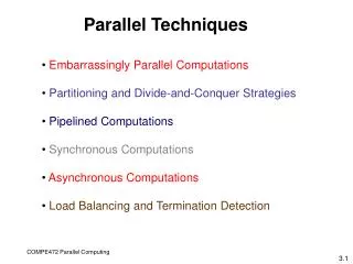
CUDA Lecture 9 Partitioning and Divide-and-Conquer Strategies. Prepared 8/19/2011 by T. O’Neil for 3460:677, Fall 2011, The University of Akron. Overview. Partitioning : simply divides the problem into parts Divide-and-Conquer :

E N D
CUDA Lecture 9Partitioning and Divide-and-Conquer Strategies Prepared 8/19/2011 by T. O’Neil for 3460:677, Fall 2011, The University of Akron.
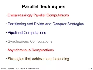
Overview • Partitioning: simply divides the problem into parts • Divide-and-Conquer: • Characterized by dividing the problem into sub-problems of same form as larger problem. Further divisions into still smaller sub-problems, usually done by recursion. • Recursive divide-and-conquer amenable to parallelization because separate processes can be used for divided parts. Also usually data is naturally localized. Partitioning and Divide-and-Conquer Strategies – Slide 2
Topic 1: Partitioning • Data partitioning/domain decomposition • Independent tasks apply same operation to different elements of a data set • Okay to perform operations concurrently • Functional decomposition • Independent tasks apply different operations to different data elements • Statements on each line can be performed concurrently Partitioning and Divide-and-Conquer Strategies – Slide 3
Example: Data Clustering • Data mining: looking for meaningful patterns in large data sets • Data clustering: organizing a data set into clusters of “similar” items • Data clustering can speed retrieval of related items Partitioning and Divide-and-Conquer Strategies – Slide 4
High-Level Document Clustering Algorithm • Compute document vectors • Choose initial cluster centers • Repeat • Compute performance function • Adjust centers until function value converges or the maximum number of iterations have elapsed • Output cluster centers Partitioning and Divide-and-Conquer Strategies – Slide 5
Data Parallelism Opportunities • Operations being applied to a data set • Examples • Generating document vectors • Finding closest center to each vector • Picking initial values of cluster centers Partitioning and Divide-and-Conquer Strategies – Slide 6
Functional Parallelism Opportunities Build document vectors Choose cluster centers Do in parallel Compute function value Adjust cluster centers Output cluster centers Partitioning and Divide-and-Conquer Strategies – Slide 7
Partitioning/Divide-and-Conquer Examples • Many possibilities: • Operations on sequences of numbers such as simply adding them together. • Several sorting algorithms can often be partitioned or constructed in a recursive fashion. • Numerical integration • N-body problem Partitioning and Divide-and-Conquer Strategies – Slide 8
Example 1: Adding a Number Sequence • Partition sequence into parts and add them. Partitioning and Divide-and-Conquer Strategies – Slide 9
Outline of CUDA Solution Partitioning and Divide-and-Conquer Strategies – Slide 10
Example 2: Bucket sort • One “bucket” assigned to hold numbers that fall within each region. • Numbers in each bucket sorted using a sequential sorting algorithm. Partitioning and Divide-and-Conquer Strategies – Slide 11
Bucket sort (cont.) • Sequential sorting time complexity: O(n log n/m) for n numbers divided into m parts. • Works well if the original numbers uniformly distributed across a known interval, say 0 to a-1. • Simple approach to parallelization: assign one processor for each bucket. Partitioning and Divide-and-Conquer Strategies – Slide 12
Example 3: Gravitational N-Body Problem • Finding positions and movements of bodies in space subject to gravitational forces from other bodies using Newtonian laws of physics. Partitioning and Divide-and-Conquer Strategies – Slide 13
Gravitational N-Body Problem (cont.) • Gravitational force F between two bodies of masses maand mb is • G is the gravitational constant and r the distance between the bodies. Partitioning and Divide-and-Conquer Strategies – Slide 14
Gravitational N-Body Problem (cont.) • Subject to forces, body accelerates according to Newton’s second law: F = mawhere m is mass of the body, F is force it experiences and a is the resultant acceleration. • Let the time interval be t. Let vt be the velocity at time t. For a body of mass m the force is Partitioning and Divide-and-Conquer Strategies – Slide 15
Gravitational N-Body Problem (cont.) • New velocity then is • Over time interval t position changes by where xt is its position at time t. • Once bodies move to new positions, forces change and computation has to be repeated. Partitioning and Divide-and-Conquer Strategies – Slide 16
Sequential Code • Overall gravitational N-body computation can be described as Partitioning and Divide-and-Conquer Strategies – Slide 17
Parallel Code • The sequential algorithm is an O(N²) algorithm (for one iteration) as each of the N bodies is influenced by each of the other N – 1 bodies. • Not feasible to use this direct algorithm for most interesting N-body problems where N is very large. • Time complexity can be reduced using observation that a cluster of distant bodies can be approximated as a single distant body of the total mass of the cluster sited at the center of mass of the cluster. Partitioning and Divide-and-Conquer Strategies – Slide 18
Barnes-Hut Algorithm • Start with whole space in which one cube contains the bodies (or particles). • First this cube is divided into eight subcubes. • If a subcube contains no particles, the subcube is deleted from further consideration. • If a subcube contains one body, subcube is retained. • If a subcube contains more than one body, it is recursively divided until every subcube contains one body. Partitioning and Divide-and-Conquer Strategies – Slide 19
Barnes-Hut Algorithm (cont.) • Creates an octtree – a tree with up to eight edges from each node. • The leaves represent cells each containing one body. • After the tree has been constructed, the total mass and center of mass of the subcube is stored at each node. • Force on each body obtained by traversing tree starting at root, stopping at a node when the clustering approximation can be used, e.g. when r d/ where is a constant typically 1.0 or less. • Constructing tree requires a time of O(n log n), and so does computing all the forces, so that the overall time complexity of the method is O(n log n). Partitioning and Divide-and-Conquer Strategies – Slide 20
Recursive division of 2-dimensional space Partitioning and Divide-and-Conquer Strategies – Slide 21
Orthogonal Recursive Bisection • (For 2-dimensional area) First a vertical line is found that divides area into two areas each with an equal number of bodies. For each area a horizontal line is found that divides it into two areas each with an equal number of bodies. Repeated as required. Partitioning and Divide-and-Conquer Strategies – Slide 22
Partitioning • Assume one task per particle • Task has particle’s position, velocity vector • Iteration • Get positions of all other particles • Compute new position, velocity Partitioning and Divide-and-Conquer Strategies – Slide 23
Final Example: Numerical Integration • Suppose we have a function ƒ which is continuous on [,b] and differentiable on (,b). We wish to approximate ƒ(x)dx on [,b]. • This is a definite integral and so is the area under the curve of the function. • We simply estimate this area by simpler geometric objects. • The process is called numerical integration or numerical quadrature. Partitioning and Divide-and-Conquer Strategies – Slide 24
Numerical Integration Using Rectangles • Each region calculated using an approximation given by rectangles; aligning the rectangles: Partitioning and Divide-and-Conquer Strategies – Slide 25
Numerical Integration Using Rectangles (cont.) • The area of the rectangles is the length of the base times the height. • As we can see by the figure base = , while the height is the value of the function at the midpoint of p and q, i.e. height = ƒ(½(p+q)). • Since there are multiple rectangles, designate the endpoints by x0 = , x1 = p, x2 = q, x3, …, xn= b; Thus Partitioning and Divide-and-Conquer Strategies – Slide 26
Example : Calculating • Can show that • Divide the interval [0,1] into the N subintervals [i-1/N,i/N] for i=1,2,3,…,N. Then Partitioning and Divide-and-Conquer Strategies – Slide 27
Simple CUDA program to compute Partitioning and Divide-and-Conquer Strategies – Slide 28
Simple CUDA program to compute (cont.) Partitioning and Divide-and-Conquer Strategies – Slide 29
Numerical integration using trapezoidal method • May not be better! Partitioning and Divide-and-Conquer Strategies – Slide 30
Numerical integration using trapezoidal method (cont.) • The area of the trapezoid is the area of the triangle on top plus the area of the rectangle below. • For the rectangle, we can see by the figure that base = , while the height = ƒ(p); thus area = ·ƒ(p). • For the triangle, base = while the height = ƒ(q) – ƒ(p), so area = ½·(ƒ(q) – ƒ(p)). Partitioning and Divide-and-Conquer Strategies – Slide 31
Numerical integration using trapezoidal method (cont.) • Thus the total area of the trapezoid is ½·(ƒ(p)+ƒ(q)). • As before there are multiple trapezoids so designate the endpoints by x0 = , x1 = p, x2 = q, x3, …, xn= b. • Thus Partitioning and Divide-and-Conquer Strategies – Slide 32
Example : Calculating • Returning to our previous example we see that Partitioning and Divide-and-Conquer Strategies – Slide 33
Example : Calculating (cont.) • Comparing our methods Partitioning and Divide-and-Conquer Strategies – Slide 34
Adaptive Quadrature • Solution adapts to shape of curve. Use three areas A, B and C. Computation terminated when largest of A and B sufficiently close to sum of remaining two areas. Partitioning and Divide-and-Conquer Strategies – Slide 35
Adaptive quadrature with false termination • Some care might be needed in choosing when to terminate. • Might cause us to terminate early, as two large regions are the same (i.e. C=0). Partitioning and Divide-and-Conquer Strategies – Slide 36
Alternate Adaptive Quadrature Algorithm • For this example we consider an adaptive trapezoid method. • Let T(,b) be the trapezoid calculation on [,b], i.e. T(,b) = ½(b-)(ƒ()+ƒ(b)). • Specify a level of tolerance > 0. Our algorithm is then: • Compute T(,b) and T(,m)+T(m,b) where m is the midpoint of [,b], i.e. m = ½(+b). • If | T(,b) – [T(,m)+T(m,b)] | < then use T(,m)+T(m,b) as our estimate and stop. • Otherwise separately approximate T(,m) and T(m,b) inductively with a tolerance of ½. Partitioning and Divide-and-Conquer Strategies – Slide 37
Example • Clearly xdx over [0,1] is 2/3. Try to approximate this with a tolerance of 0.005. • In this case T(,b) = ½(b – )( + b). • T(0,1) = 0.5, tolerance is 0.005. T(0,½) + T(½,1) = 0.176777 + 0.426777 = 0.603553 |0.5 – 0.603553| = 0.103553; try again. • Estimate T(½,1) with tolerance 0.0025. T(½,¾) + T(¾,1) = 0.196642 + 0.233253 = 0.429895 |0.426777 – 0.429895| = 0.003118; try again. Partitioning and Divide-and-Conquer Strategies – Slide 38
Example (cont.) • Estimate T(½, ¾) and T(¾,1) each with tolerance 0.00125. • T(½, ¾) = 0.196642. T(½, ⁵⁄₈) + T(⁵⁄₈, ¾) = 0.093605 + 0.103537 = 0.197142. |0.196642 – 0.197142| = 0.0005; done. • T(¾, 1) = 0.233253. T(¾, ⁷⁄₈) + T(⁷⁄₈, 1) = 0.112590 + 0.120963 = 0.233553. |0.233253 – 0.233553| = 0.0003; done. • Our revised estimate for T(½,1) is the sum of the revised estimates for T(½, ¾) and T(¾, 1). • Thus T(½,1) = 0.197142 + 0.233553 = 0.430695. Partitioning and Divide-and-Conquer Strategies – Slide 39
Example (cont.) • Now for T(0,½). Partitioning and Divide-and-Conquer Strategies – Slide 40
Example (cont.) • Still more for T(0,½). Partitioning and Divide-and-Conquer Strategies – Slide 41
Example (cont.) • So our final estimate for T(0,½) is 0.235113. • Our previous final estimate for T(½,1) was 0.430695. • Thus the final estimate for T(0,1) is the sum of those for T(0,½) and T(½,1) which is 0.665808. • The actual answer was 2/3 for an error of 0.0008586, well below our tolerance of 0.005. Partitioning and Divide-and-Conquer Strategies – Slide 42
Summary • Two strategies • Partitioning: simply divides the problem into parts • Divide-and-Conquer: divide the problem into sub-problems of same form as larger problem • Examples • Operations on sequences of numbers such as simply adding them together. • Several sorting algorithms can often be partitioned or constructed in a recursive fashion. • Numerical integration • N-body problem Partitioning and Divide-and-Conquer Strategies – Slide 43
End Credits • Based on original material from • The University of Akron: Tim O’Neil • The University of North Carolina at Charlotte • Barry Wilkinson, Michael Allen • Oregon State University: Michael Quinn • Revision history: last updated 8/19/2011. Partitioning and Divide-and-Conquer Strategies – Slide 44