Download
1 / 31
310 likes | 436 Vues
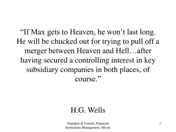
“If Max gets to Heaven, he won’t last long. He will be chucked out for trying to pull off a merger between Heaven and Hell…after having secured a controlling interest in key subsidiary companies in both places, of course.”. H.G. Wells. The Impact of Unanticipated Changes in Interest Rates:.

E N D
“If Max gets to Heaven, he won’t last long. He will be chucked out for trying to pull off a merger between Heaven and Hell…after having secured a controlling interest in key subsidiary companies in both places, of course.” H.G. Wells Saunders & Cornett, Financial Institutions Management, 4th ed.
The Impact of Unanticipated Changes in Interest Rates: • On Profitability • Net Interest Income (NII) = Interest Income minus Interest Expense • Interest rate risk of NII is measured by the repricing model. (chap. 8) • On Market Value of Equity • Market Value of Equity = Market Value of Assets minus Market Value of Debt • Interest rate risk of equity MV is measured by the duration model. (chap. 9) Saunders & Cornett, Financial Institutions Management, 4th ed.
The Repricing Model • Rate Sensitive Assets (Liabilities) RSA/RSL: are repriced within a period of time called a maturity bucket. • Repricing occurs whenever either maturity or a roll date is reached. • The roll date is the reset date specified in floating rate instruments that determines the new market benchmark rate used to set cash flows (eg., coupon payments). • The Federal Reserve set the following 6 maturity buckets: 1 day; 1day-3 months; 3-6 months; 6-12 months; 1-5 yrs; > 5 yrs. Saunders & Cornett, Financial Institutions Management, 4th ed.
The Repricing Model • Repricing Gap (GAP) = RSA – RSL • R = interest rate shock • NII = GAP x R for each maturity bucket i • Cumulative Gap (CGAP) = i GAPi • NII = CGAP x Ri where Ri is the average interest rate change on RSA & RSL • Gap Ratio = CGAP/Assets Saunders & Cornett, Financial Institutions Management, 4th ed.
Example of Repricing Model Saunders & Cornett, Financial Institutions Management, 4th ed.
Repricing Ex. (cont.) • 1 day GAP = 0 – 0 = 0 (DD & passbook excluded) • (1day-3mo] GAP = 30 – (40+20) = -$30m • (3mo-6mo] GAP = 35 – 60 = -$25m • (6mo-12mo] GAP = (50+40) - 20 = $70m • (1yr-5yr] GAP = (25+70) – 40 = $55m • >5 yr GAP = 20 – (20+40+30) = -$70m • 1 yr CGAP = 0-30-25+70 = $15m • 1 yr Gap Ratio = 15/270 = 5.6% • 5 yr CGAP = 0-30-25+70+55 = $70m • 5 yr Gap Ratio = 70/270 = 25.9% Saunders & Cornett, Financial Institutions Management, 4th ed.
Assume an across the board 1% increase in interest rates • 1 day NII = 0(.01) = 0 • (1day-3mo] NII = -$30m(.01) = -$300,000 • (3mo-6mo] NII = -$25m(.01) = -$250,000 • (6mo-12mo] NII = $70m(.01) = $700,000 • (1yr-5yr] NII = $55m(.01) = $550,000 • >5 yr GAP = -$70m(.01) = -$700,000 • 1 yr CNII = $15m(.01) = $150,000 • 5yr CNII = $70m(.01) = $700,000 Saunders & Cornett, Financial Institutions Management, 4th ed.
Unequal Shifts in Interest Rates • NII = (RSA x RRSA) – (RSL x RRSL) • Even if GAP=0 (RSA=RSL) unequal shifts in interest rates can cause NII. • Must compare relative size of RSA and RSL (GAPs) to relative size of interest rate shocks (RRSA- RRSL = spread). • The spread can be positive or negative = Basis Risk. Saunders & Cornett, Financial Institutions Management, 4th ed.
Strengths of Repricing Model • Simplicity • Low data input requirements • Used by smaller banks to get an estimate of cash flow effects of interest rate shocks. Saunders & Cornett, Financial Institutions Management, 4th ed.
Weaknesses of the Repricing Model • Ignores market value effects. • Overaggregation within maturity buckets • Runoffs – even fixed rate instruments pay off principal and interest cash flows which must be reinvested at market rates. Must estimate cash flows received or paid out during the maturity bucket period. But assumes that runoffs are independent of the level of interest rates. Not true for mortgage prepayments. • Ignores cash flows from off-balance sheet items. Usually are marked to market. Saunders & Cornett, Financial Institutions Management, 4th ed.
Measuring the Impact of Unanticipated Interest Rate Shocks on Market Values • E = A - L • What determines price sensitivity to changes in interest rates? • The longer the time to maturity, the greater the price impact of any given interest rate shock. • This can be viewed in the positively sloped yield curve. See Appendix 8A. • But, yield curves must be drawn using pure discount yields. • The correct statement is: The longer the DURATION, the greater the price impact of any given interest rate shock. Saunders & Cornett, Financial Institutions Management, 4th ed.
What is Duration? • Duration is the weighted-average time to maturity on an investment. • Duration is the investment’s interest elasticity - measures the change in price for any given change in interest rates. • Duration (D) equals time to maturity (M) for pure discount instruments only. • Duration of Floating Rate Instrument = time to first roll date. • For all other instruments, D < M • Duration decreases as: • Coupon payments increase • Time to maturity decreases • Yields increase. Saunders & Cornett, Financial Institutions Management, 4th ed.
The Spreadsheet Method of Calculating DurationEx. 1:5 yr. 10% p.a. coupon par value Saunders & Cornett, Financial Institutions Management, 4th ed.
Ex. 2: Interest Rates Decrease to 9% p.a. Saunders & Cornett, Financial Institutions Management, 4th ed.
Ex. 3: Interest Rates Increase to 11% p.a. Saunders & Cornett, Financial Institutions Management, 4th ed.
The Duration Model • Modified Duration = MD = D/(1+R) • Price sensitivity (interest elasticity): P -D(P)R/(1+R) • Consider a 1% increase in interest rates: • Ex. 1: P -(4.17)(1000)(.01)/1.10 = -$37.91 - New Price = 1000 - 37.91 = $962.09 Exact $963.04 • Ex. 2: P -(4.19)(1038.897)(.01)/1.09 = -$39.94 • New Price = 1038.897 – 39.94 = $998.96 Exact $1000 • Ex. 3: P -(4.15)(963.041)(.01)/1.11 = -$36.01 • New Price = 963.041 – 36.01 = $927.03 Exact $927.90 Saunders & Cornett, Financial Institutions Management, 4th ed.
The Duration Model: Using Duration to Measure the FI’s Interest Rate Risk Exposure • E = A - L • A = -(DAA)RA/(1+RA) • L = -(DLL)RL/(1+RL) • Assume that RA/(1+RA) = RL/(1+RL) • E/A -DG(R)/(1+R) where • DG = DA – (L/A)DL • DA = i=A wiDi DL = j=L wjDj Saunders & Cornett, Financial Institutions Management, 4th ed.
Consider a 2% increase in all interest rates (ie, R/(1+R) = .02) • FI with DG = +5 yrs. E/A -10% • FI with DG = +2 yrs. E/A -4% • FI with DG = +0.5 yrs E/A -1% • FI with DG = 0 E/A 0% Immunization • FI with DG = -0.5 yrs E/A +1% • FI with DG = - 2 yrs E/A +4% • FI with DG = - 5 yrs E/A +10% Saunders & Cornett, Financial Institutions Management, 4th ed.
Convexity • Second order approximation • Measures curvature in the price/yield relationship. • More precise than duration’s linear approximation. • Duration is a pessimistic approximator • Overstates price declines and understates price increases. • Convexity adjustment is always positive. • Long term bonds have more convexity than short term bonds. Zero coupon less convex than coupon bonds of same duration. P -D(P)(R)/(1+R) + .5(P)(CX)(R)2 Saunders & Cornett, Financial Institutions Management, 4th ed.
The Spreadsheet Method to Calculate Convexity Ex. 1 Saunders & Cornett, Financial Institutions Management, 4th ed.
Ex. 2 Saunders & Cornett, Financial Institutions Management, 4th ed.
Ex. 3 Saunders & Cornett, Financial Institutions Management, 4th ed.
How Do We Forecast Interest Rate Shocks? • Expectation Hypothesis • Upward (downward) sloping yield curve forecasts increasing (decreasing) interest rates. • (1+0R2)2 = (1+0R1)(1+1R1) • Spot rates: 0R2= 5.5% p.a. 0R1=4% Implied forward rate: 1R1 = 7.02% p.a. Forecasts 3.02% increase in 1 yr rates in 1 yr. • Liquidity Premium Hypothesis • Market Segmentation Hypothesis Saunders & Cornett, Financial Institutions Management, 4th ed.
Appendix 8A Calculating the Forward Zero Yield Curve for Valuation • Three steps: • Decompose current spot yield curve on risk-free (US Treasury) coupon bearing instruments into zero coupon spot risk-free yield curve. • Calculate one year forward risk-free yield curve. • Add on fixed credit spreads for each maturity and for each credit rating. Saunders & Cornett, Financial Institutions Management, 4th ed.
Step 1: Calculation of the Spot Zero Coupon Risk-free Yield Curve Using a No Arbitrage Method • Figure 6.6 shows spot yield curve for coupon bearing US Treasury securities. • Assuming par value coupon securities: • Figure 6.7 shows the zero coupon spot yield curve. Saunders & Cornett, Financial Institutions Management, 4th ed.
Saunders & Cornett, Financial Institutions Management, 4th ed.
Step 2: Calculating the Forward Yields • Use the expectations hypothesis to calculate 6 month maturity forward yields: Saunders & Cornett, Financial Institutions Management, 4th ed.
Use the 6 month maturity forward yields to calculate the 1 year forward risk-free yield curve Figure 6.8 Saunders & Cornett, Financial Institutions Management, 4th ed.
Step 3: Add on Credit Spreads to Obtain the Risky 1 Year Forward Zero Yield Curve • Add on credit spreads (eg., from Bridge Information Systems) to obtain FYCR in Figure 6.8. Saunders & Cornett, Financial Institutions Management, 4th ed.
Calculating Duration if the Yield Curve is not FlatEx. 1 with upward sloping yield curve Saunders & Cornett, Financial Institutions Management, 4th ed.
The Barbell Strategy • Convexity of Zero Coupon Securities: CX = T(T+1)/(1+R)2 • Strategy 1: Invest in 15 yr zero coupon with 8% pa yield. D=15, CX = 15(16)/1.082=206 • Strategy 2: Invest 50% in overnite FF D=0, CX =0 and 50% in 30 yr zero coupon with 8% yield D=30, CX = 30(31)/1.082 = 797 Portfolio CX = .5(0) + .5(797) = 398.5 > 206 Invest in Strategy 2. But the cost of Strategy 2>Stategy 1 if CX priced. Saunders & Cornett, Financial Institutions Management, 4th ed.