Download
1 / 20
200 likes | 223 Vues
This article provides an overview of descriptive statistics, measurement scales, and techniques for analyzing and interpreting data. Topics covered include summation notation, percentiles, measures of central tendency, variability, and standard deviation. The article also discusses standard scores, their use in comparing scores from different scales, and the normal distribution of scores.

E N D
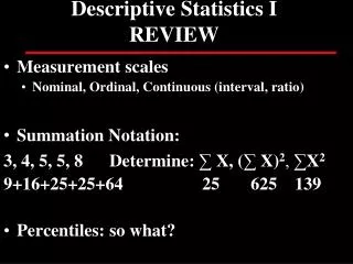
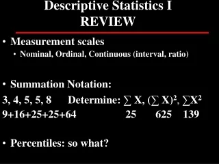
Descriptive Statistics IREVIEW • Measurement scales • Nominal, Ordinal, Continuous (interval, ratio) • Summation Notation: 3, 4, 5, 5, 8 Determine: ∑ X, (∑ X)2, ∑X2 9+16+25+25+64 25 625 139 • Percentiles: so what?
Measures of central tendency • Mean, median mode • 3, 4, 5, 5, 8 • Distribution shapes
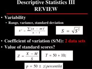
Total variance Variability • RangeHi – Low scores only (least reliable measure; 2 scores only) • Variance (S2)Spread of scores based on the squared deviation of each score from mean Most stable measure • Standard DeviationThe square root of the variance Most commonly used measure of variability Error TrueVariance
Variance (Table 3.2) The didactic formula 4+1+0+1+4=1010 = 2.5 5-1=4 4 The calculating formula 55 - 225 = 55-45=10 = 2.5 5 4 4 4
Standard Deviation The square root of the variance Nearly 100% scores in a normal distribution are captured by the mean + 3 standard deviations
The Normal Distribution M + 1s = 68.26% of observations M + 2s = 95.44% of observations M + 3s = 99.74% of observations
Calculating Standard Deviation Raw scores 3 7 4 5 1 ∑ 20 Mean: 4 (X-M) -1 3 0 1 -3 0 (X-M)2 1 9 0 1 9 20 S= √20 5 S= √4 S=2
Coefficient of Variation (V) Relative variability around the mean OR Determines homogeneity of scores S M Helps more fully describe different data sets that have a common std deviation (S) but unique means (M) Lower V=mean accounts for most variability in scores .1 - .2=homogeneous >.5=heterogeneous
Descriptive Statistics II • What is the “muddiest” thing you learned today?
Descriptive Statistics IIREVIEW Variability • Range • Variance: Spread of scores based on the squared deviation of each score from mean Most stable measure • Standard deviation Most commonly used measure Coefficient of variation • Relative variability around the mean (homogeneity of scores) • Helps more fully describe different data sets that have a common std deviation (S) but unique means (M) 50+10 • What does this tell you?
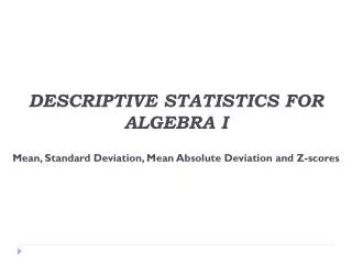
Standard Scores • Set of observations standardized around a given M and standard deviation • Score transformed based on its magnitude relative to other scores in the group • Converting scores to Z scores expresses a score’s distance from its own mean in sd units • Use of standard scores: determine composite scores from different measures (bball: shoot, dribble); weight?
Standard Scores • Z-score M=0, s=1 • T-scoreT = 50 + 10 * (Z) M=50, s=10
Conversion to Standard Scores Raw scores 3 7 4 5 1 • Mean: 4 • St. Dev: 2 X-M -1 3 0 1 -3 Z -.5 1.5 0 .5 -1.5 SO WHAT? You have a Z score but what do you do with it? What does it tell you? Allows the comparison of scores using different scales to compare “apples to apples”
Normal-curve Areas Table 3-3 • Z scores are on the left and across the top • Z=1.64: 1.6 on left , .04 on top=44.95 • Values in the body of the table are percentage between the mean and a given standard deviation distance • The "reference point" is the mean
Area of normal curve between 1 and 1.5 std dev above the mean Figure 3.9
Normal curve practice • Z score Z = (X-M)/S • T score T = 50 + 10 * (Z) • Percentile P = 50 + Z percentile(+: add to 50, -: subtract from 50) • Raw scores • Hints • Draw a picture • What is the z score? • Can the z table help?
Descriptive Statistics III • Explain one thing that you learned today to a classmate • What is the “muddiest” thing you learned today?