Download
1 / 54
540 likes | 555 Vues
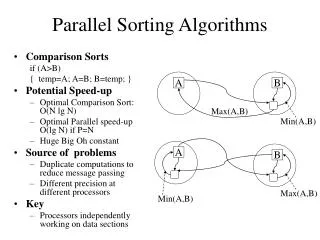
Parallel Sorting Algorithms. The simple sorting algorithms (Bubble Sort, Insertion Sort, Selection Sort, …) are Lower bound on comparison based algorithms (Merge Sort, Quicksort, Heap Sort, …) is

E N D
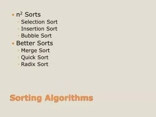
The simple sorting algorithms (Bubble Sort, Insertion Sort, Selection Sort, …) are • Lower bound on comparison based algorithms (Merge Sort, Quicksort, Heap Sort, …) is • The best we can hope to do with parallelizing a comparison-based algorithm using n processors is
Question: What can we expect if we use n2 processors? • Answer: Typically, it is still:
In place sorting – sorting the values within the same array • Not in-place (or out-of-place) sorting – sorting the values to a new array • Stable sorting algorithm – Identical values remain in the same order as the original after sorting
Compare and Exchange • Most sorting algorithms (although not all) compare two values and possibly exchange them • Two numbers in the array are compared with each other: if (A[i] > A[j]) { temp = A[i]; A[i] = A[j]; A[j] = temp; }
Message-passing Compare and Exchange (version 1) • In a distributed-memory system, we have to send message to exchange values • P1 send value to P2. P2 compares the two values; keeps the larger and sends the smaller back to P1 Processor 1 Processor 2 A[i] A[j] A[i] A[i] is sent Smaller Value Returned Larger Value Kept
Message-passing Compare and Exchange (version 2) • Both processors send their values to each other. They both compare values. P1 keeps the smaller value, P2 keeps the larger values. Processor 1 Processor 2 A[i] A[j] A[i] A[j] A[i] is sent A[j] is sent Smaller Value Kept Larger Value Kept
Message-passing Compare and Exchange (version 1) • When we have the number of values (n) is much larger than the number of processors (p), then each processors is responsible of n/p values Processor 1 Processor 2 Final Values Original Values (sorted first) 88 50 28 25 Original Values (sorted first) 98 80 43 42 merge 98 88 80 50 43 42 28 25 Larger Numbers Kept 43 42 28 25 88 50 28 25 Final Values Smaller Numbers Sent
Message-passing Compare and Exchange (version 2) • When we have the number of values (n) is much larger than the number of processors (p), then each processors is responsible of n/p values Processor 2 Processor 2 98 88 80 50 43 42 28 25 88 50 28 25 98 80 43 42 merge 98 88 80 50 43 42 28 25 merge Larger Numbers Kept Original Values sent 98 80 43 42 88 50 28 25 Smaller Numbers Kept
Bubble Sort • N passes are made comparing/exchanging adjacent values • Larger values settle to the bottom (Sediment Sort?) • After pass m, the m largest values are in the m last locations in the array.
Complexity of Bubble Sort • The number of comparison/exchanges with Bubble Sort is: • Very slow but easy to parallelize • We can use a pipeline-sort of technique
Parallel Bubble Sort P1 P2 P3 P4 P5 P6 P7 P0 Phase 1 Time Phase 2 Phase 3
Even-Odd Transposition Sort • Uses alternating even and odd phases • Even phase • even processors exchange with next higher ranked processor • odd processors exchange with the next lower ranked processor • Odd phase • even processors exchange with next lower ranked processor • odd processors exchange with the next higher ranked processor
Even-Odd Sort P1 P2 P3 P4 P5 P6 P7 P0 4 2 7 8 5 1 3 6 2 4 7 8 1 5 3 6 2 4 7 1 8 3 5 6 Time 2 4 1 7 3 8 5 6 2 1 4 3 7 5 8 6 1 2 3 4 5 7 6 8 1 2 3 4 5 6 7 8 1 2 3 4 5 6 7 8
What is the time complexity of Parallel Bubble Sort with n processors? • Answer: 2n=O(n) • What is the time complexity of Even-Odd Sort with n processors? • Answer: O(n)
Divide and Conquer Pattern • Characterized by dividing problem into sub-problems of same form as larger problem. • Further divisions into still smaller sub-problems, usually done by recursion. Creates a tree. • Recursive divide and conquer amenable to parallelization because separate processes can be used for divided parts. Also usually data becomes naturally localized.
Sorting - Several sorting algorithms can often be partitioned or constructed in a recursive divide and conquer fashion, e.g. Mergesort, Quicksort, • Searching algorithms dividing search space recursively
Merge Sort • Merge Sort is a “Divide and Conquer” algorithm • The array is divided into smaller and smaller parts • Then the small parts are merged into a new sorted sub array
Merge Sort P1 P2 P3 P4 P5 P6 P7 P0 4 2 7 8 5 1 3 6 Divide 4 2 7 8 5 1 3 6 4 2 7 8 5 1 3 6 Time 4 2 7 8 5 1 3 6 Merge 2 4 7 8 1 5 3 6 2 4 7 8 1 3 5 6 1 2 3 4 5 6 7 8
Complexity of Parallel Merge Sort • Complexity of the sequential merge sort: • Complexity of parallel merge sort with n processors • There are 2logn steps, but each merge step takes longer and longer • Turns out to be:
Quicksort • Pick a pivot • The move all the values less than the pivot to the left side of the array • And all the values greater than the pivot to the right side • Then recursively sort the two sides
Quicksort • Works well when the pivot is approximately in the middle • If the pivot is chosen poorly, quicksort resorts to
Neither Merge Sort nor Quicksort parallelize efficiently • Still • Any tree structure (reduction, merge, quicksort) cannot be parallelized by n processors efficiently
Batcher’s Parallel Sorting Algorithms • Odd-even Merge Sort (not the same as even-odd transposition sort) • Bitonic Merge Sort • Complexity with n processors:
Summary (using n processors to sort n numbers) • Parallel Bubble sort and Odd-even transposition sort - O(n) • Parallel mergesort - O(n) but unbalanced processor load and communication (because of tree) • Parallel quicksort - O(n) but unbalanced processor load and communication (because of tree) and can degenerate to O(n2) • Odd-even Mergesort - O(log2n)
Sorting on Specific Networks • Two network structures have received specific attention: • Mesh • Hypercube • because parallel computers have been built with these networks. • Of less interest nowadays because underlying architecture often hidden from user. • There are MPI features for mapping algorithms onto meshes. • Can always use a mesh or hypercube algorithm even if the underlying architecture is not the same.
Mesh - Two-Dimensional Sorting • Final sorted list -- could be row by row or snakelike.
Shearsort • Alternate row and column sorted until list fully sorted • Result is a snake-like sorting • On a mesh, this requires steps
Other Sorts(Coming Up Next) • Rank Sort • Counting Sort • Radix Sort
Rank Sort • The idea of rank sort is to count the number of values less than a[i] • That count is the “rank” of that value • The rank is where in the sorted array that value will be placed • So we can put in into that spot b[rank] = a[i].
Rank Sort (Sequential Code) for (i = 0; i < n; i++) { // for each number x = 0; for (j = 0; j < n; j++) // count number less than it if (a[i] > a[j]) x++; b[x] = a[i]; // copy number into correct place } • Doesn’t handle duplicate values (How can this be fixed?) • The complexity is O(n2) • However, this is easy to parallelize
Rank Sort (Parallel Code) forall (i = 0; i < n; i++) { // each processor allocated different value x = 0; for (j = 0; j < n; j++) // count number less than it if (a[i] > a[j]) x++; b[x] = a[i]; // copy number into correct place } • Uses n processors and complexity is O(n) • Very easy to implement in OpenMP • As good as many of the parallel sorts (except bitonic and shear sort)
Rank Sort using n2 processors • Instead of one processors comparing a[i] with other values, we use n-1 proces-sors • Incrementing counter is a critical section; must be sequential, so this is still O(n)
Rank Sort using n2 processors • Can do this as a reduction • Complexity is O(logn) with n2 processors • Low processor efficiency
Counting Sort • The best sequential sorting algorithms are O(nlogn). • We can do better if we can make assumption about the data • If the values are all integers within a relatively small range of values, we can do Counting Sort in O(n) instead of O(n2) or O(nlogn).
Counting Sort • Counting Sort is a stable sort (identical values remain in same relative position as in orginal array) • However, it is not an “in-place” sort • Further more, we need extra space • Suppose original values in the array a[ ] • Sorted array will be b[ ] • Create an array c[ ] of size m where values of a[ ] are in the range 1..m.
Counting Sort – Step 1 • c[ ] is the histogram of values in the array. In other words, it is the sum of equal values • Complexity is O(m + n) for (i = 1; i <= m; i++) c[i] = 0; for (i = 1; i <= n; i++) c[ a[i] ]++;
Counting Sort – Step 2 • We can find the rank of each value by doing a prefix sum on c[ ] for (i = 2; i <= m; i++) c[i] = c[i] + c[i-1]; • Complexity is O(m)
Counting Sort – Step 3 • We can now use the prefix sum to place the values where they should go: for (i = n; i >= 1; i--) { b[ c[ a[i] ] ] = a[i] c[ a[i] ]--; // ensures stable sorting } • Sequential complexity for all 3 steps is O(m + n) • If m is linear with n, then complexity is O(n)
Counting Sort 1 2 3 4 5 6 7 8 1 1 1 5 2 2 1 2 3 1 3 3 7 4 1 4 6 7 1 4 1 8 6 1 5 2 5 6 5 Original sequence a[] Step 3 moves backwards thro a[] Step 1. Histogram c[] Step 2. Prefix sum c[] Move 5 to position 6. Then decrement c[5] b[] 7 Step 3. Sort Final sorted sequence
Parallel Counting Sort (using n processors) • Step 1 – Creating the Histogram: O(logn). We use the same tree as with rank sort. Updating c[a[i]]++ is a critical section when there are duplicate values in a[ ]. • Step 2 – Parallel version of prefix sum using n processors is O(logn) • Step 3 – Placing number in place: O(logn) again because of possible duplicate values (c[a[i]]– is a critical section) • All 3 steps: O(logn)
Radix Sort • Assumption: Values are either unsigned decimal or unsigned binary • Sort values based on least significant digit • Then sort on next least significant digit • Continue until the most significant digit is used to sort. • This works if we use a stable sorting algorithm • Since each digit will be in the range 0-9 or 0-1, then we can use Counting Sort for each digit