Computational Physics Numerical Integration
310 likes | 676 Vues
Computational Physics Numerical Integration. Dr. Guy Tel- Zur. Tulips by Anna Cervova , publicdomainpictures.net. MHJ- Chap. 7 – Numerical Integration. Agenda 1D integration (Trapezoidal and Simpson rules) Gaussian quadrature (when the abscissas are not equally spaced)

Computational Physics Numerical Integration
E N D
Presentation Transcript
Computational PhysicsNumerical Integration Dr. Guy Tel-Zur Tulips by Anna Cervova, publicdomainpictures.net
MHJ- Chap. 7 – Numerical Integration • Agenda • 1D integration (Trapezoidal and Simpson rules) • Gaussian quadrature (when the abscissas are not equally spaced) • Singular integrals • Physics case study • Parallel Computing (part 1)
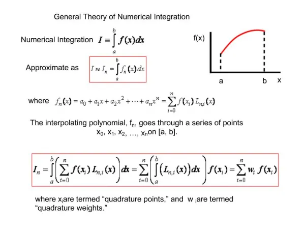
Newton-Cotes quadrature: equal step methods Step size:
The strategy then is to find a reliable Taylor expansion for f(x) in the smaller sub intervals 7.2 Let’s define x0 = a + h and use x0 as the midpoint. The general form for the Taylor expansion around x0 goes like:
Let us now suppose that we split the integral in Eq. (7.2) in two parts, one from x0−h to x0 and the other from x0 to x0 + h, that is, our integral is rewritten as: Next we assume that we can use the two-point formula for the derivative, meaning that we approximate f(x) in these two regions by a straight line, as indicated in the figure. This means that every small element under the function f(x) looks like a trapezoid. we are trying to approximate our function f(x) with a first order polynomial, that is f(x) = a + bx. The constant b is the slope given by the first derivative at x = x0:
Trapezoidal Rule • A worked out example in “C”. • We will learn how to Integrate a general form of a function? • The code is under: lecture02/code_ch_07/trapez.c
// Computational Physics // Guy Tel-Zur, August 2010 // Trapezoidal Rule // Based on MHJ Page 129, Chapter 7, 2009 Fall Edition // Usage: standard gcc -o fnfn.c -lm #include <math.h> #include<stdio.h> int main() { // functions declarations: double TrapezoidalRule(double a , double b , int n, double(*func )(double)); double MyFunction(double x); // variables declarations: double a = 0.0; double b = 10.0; int n = 1000; double s; s = TrapezoidalRule(a, b, n, &MyFunction); printf("Trapezoidal Rule Integral=%Lf\n",s); return 0; } // end of main
double TrapezoidalRule (double a , double b , int n, double(*func )(double)) { double TrapezSum; double fa ,fb ,x ,step ; int j; step =(b-a)/((double)n ); fa =(*func)(a)/2.; fb =(*func)(b)/2.; TrapezSum= 0.; for(j=1;j<=n-1;j++) { x=j*step+a; TrapezSum+=(*func)(x); } TrapezSum=(TrapezSum+fb+fa)*step; return TrapezSum; } // end TrapezoidalRule double MyFunction(double x) { // write below the mathematical expression of the // function to be integrated return x*x; }
Section 7.5 – Rectangle Rule Another very simple approach is the so-called midpoint or rectangle method. In this case the integration area is split in a given number of rectangles with length h and height given by the mid-point value of the function. This gives the following simple rule for approximating an integral • Demo: ch7 code folder. Program: rectangle_trapez.c double RectangleRule (double a , double b , int n, double(*func )(double)) { double RectangleSum; double fa ,fb ,x ,step ; int j; step =(b-a)/((double)n ); RectangleSum= 0.; for(j=0;j<=n;j++) { x=(j+0.5)*step+a; RectangleSum+=(*func)(x); } RectangleSum *= step; return RectangleSum; } // end Rectangle Rule
Error analysis • Trapezoidal & Rectangle rules: • Local error: α h^3 • Global error: α h^2 • Global error: α (b-a)
Can’t we do better? • So far: Linear two-points approximations for f • Now (Simpson’s): three-points formula (a parabola): • Recall from Chapter 3, the 1st and the 2nd derivatives approximations: • f’= • f’’=
With the latter two expressions we can now approximate the function f as: I gave up using Equation Editor – Sorry… Next Slide…
Note that the improved accuracy in the evaluation of the derivatives gives a better error approximation, O(h5) vs. O(h3) . - This is the local error. The global error goes like: O(h4). The full integral is therefore:
7.3 Adaptive Integration • Naïve approach, for example, two parts of Trapezoidal Integration with a different step size
7.4 Gaussian Quadrature (GQ) We could fit a polynomial of order N with N equally spaced points, but Gauss, who was a genius, suggested to fit a polynomial of order 2N-1 with N points!!!
Recommended online video: http://physics.orst.edu/~rubin/COURSES/VideoLecs/Integration/Integration.html
Speaking about references, you can always check Google Books http://www.google.com/search?tbs=bks%3A1&tbo=1&q=computational+physics&btnG=Search+Books
Another recommended reference: Computational Physics By Steven E. Koonin So far – equally spaced points: Our derivation is exact if f is polynomial 4.9 Note: This is a set of N linear equations (for each p) !!!
Sage demo • Upload: “Gaussian Quadrature Demo.sws” • Reference: http://wiki.sagemath.org/interact/calculus
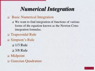
Let’s sum what we did so far 2 points integration: Trapezoidal Rule (+Rectangle Rule),fit straight line 3 points integration: Simpson’s Rule, fit a parabola Quadrature Formula: Gauss Quadrature:
The program1.cpp is a ready for comparing the 3 integrations methods mentioned. The Trapezoidal, Simpson’s and GQ function are to be written. >> Explain this program (open DevC++ IDE)