Download
1 / 17
170 likes | 305 Vues
GENERALIZATION OF THE METHOD OF FINIT E DIFFERENCES. ARYASSOV, Gennady BARASKOVA, Tatjana GORNOSTAJEV, Dmitri PETRITSHENKO, Andres Tallinn University of Technology.

E N D
GENERALIZATION OF THE METHOD OF FINITE DIFFERENCES ARYASSOV, Gennady BARASKOVA, Tatjana GORNOSTAJEV, DmitriPETRITSHENKO, Andres Tallinn University of Technology
The theory of the method of finite differences is based on the theory of the approximation of functions, when values of them in discrete points are known. For this purpose, the interpolation polynomials obtained by the method of the uncertain coefficients are applied. Such approximation is possible to execute without resorting to the finite difference schemes (Jensen, 1972). The method of uncertain coefficient can be used as for the traditional method of grids as for the “improved method of grids", which has been developed (Kollats, 1969) for solution of partial differential equations especially. The method of grids allows to reduce a task of continuous analysis to a problem of solution of system of the algebraic equations. The accuracy of the used interpolation polynomials is established by the well-known formulas from literature. 1. Motivation(Introduction)
y y f (x) y0 y1 y2 y3 yn-1 yn-2 yn x . . . n a n - 2 n - 1 b 3 1 2 Let's consider the closed interval [a,b] shown in Fig.1 and which is a part of wider interval [A,B]. We set a task to approach the given function y=f(x) by the method of uncertain coefficients. The arbitrarily located interval [a,b], along an axis х with length l=b-a, is divided to n equal parts with length h=(b-a)/n. 2. Approximation by method of uncertain coefficients Fig. 1. The closed interval of [a,b]
It is required to find interpolationpolynomial coefficients Pn(x) of degree n which graph passes consistently one time through all values yi, i = 0, 1, 2, …, nand only once. With the help of the formulas (2) it is possible to make transfer of a beginning of coordinates to apoint х=a, that is to change scale on an axis х. After replacement of arguments х in the interpolation polynomial (1) to dimensionless we receive The mutual transition from the polynomial (1) to the polynomial (3) and back is carried out with the help of the transformation formula (2). It is possible to write down the polynomial in matrix notable (symbolic) as follows
The mutual transition from the polynomial (1) to the polynomial (3) and back is carried out with the help of the transformation formula (2). It is possible to write down the polynomial in matrix notable (symbolic) as follows SubstitutinginthepolynomialPn*(ξ)the integer values of dimensionless argument and appropriate values of function y, the following system of the equations for calculation coefficients is obtained which can be written down in a matrix form
where [Wn] - Vandermode matrix, which elements are degrees of a natural line numbers. The Vandermode matrix is not particular, therefore finding the inverse matrix to it is not difficult task and does not require the large efforts. Multiplying the equation (6) at the left on [Wn]-1the line of coefficients is determined Substituting expression (7) in the formula (4) we can present interpolation polynomials in the matrix form
y y=0 P4*(ξ)= -10 +17 2-8 3+4 y1= 0 y0= 0 3 4 2 0 1 y2= 0 y3=12 y = -12 (-2) y4=24 Example. Approximate a broken line consisting of straight lines y = 0 and y = -12 (x - 2),by the fourth degree polynomial (Fig.2). Fig. 2. The interpolation of broken line As the matrix [Wn]-1is multiplied on 4!, the coefficients then should be divided on 4! =24.
y a, b a, b y1* y3* y0* y2* y0 y1 y2 y3 y4 y 0 1 5 7 4 2 6 3 a, b a1, b1 In case of approximation of function on the extended interval [A,B], which can consist of several intervals of a type [a,b], are used the earlier received formulae. It is allowed, that intervals [a,b] can overlap each other or be imposed against each other. On Fig.3 one of such possible cases is shown. Fig.3. Approximation of function on the extended interval [A,B]
The corresponding to an interval [a,b] ordinates are denoted у0, у1, …, уn. The corresponding to the next interval [a,b] ordinates are denoted The ordinates and coincide both on the location and on size. Intermediate ordinate in area, where there is "overlapping (Fig.3) is possible to receive by two ways: • substituting in interpolation polynomials a value from the interval [a,b], • substituting ininterpolation polynomials value from the interval [a,b] *. • In general case the given substitutions give various, but close results, this is explained by inexactitude of interpolation formulae. It is known, that the error of interpolation formulae is less in middle of an interval of interpolation and is great outside of it. In particular it is necessary to take into account this circumstance in calculation a derivative. Therefore it is expedient to use overlapping of intervals, especially, if the high order derivatives are to be calculated. • It should be noticed, that the beginning of coordinates of interpolation polynomials can be changed arbitrarily, but to change the order of following of nodes and corresponding ordinates is not allowed in any event .
From the formula (3) follows, that for calculation a derivative of interpolation polynomial is sufficient to differentiate only matrix-line {ξ}T. Other multipliers of expression (8) are invariant to operation of differentiation. Above-mentioned statement in identical degree concerns to operation of integration. For example, third derivative from the polynomial (8) will be defined as 3. Interpolation of Derived Function (Derivatives) It is possible with the help of the formula (9) to calculate derivative value in any point of the interval [a,b]. For example, at ξ = 1 the third derivative value is equal
It is important to know in the method of grids the derivative values in nodes of interpolation. These values are easy obtained from the formulae (12) if suppose, that accepts consistently the values as: = 0, 1, 2, …, n. Then the line of mth derivative from [ξ]T becomes a square matrix. At n = 4 matrixes - columns or the vector - column second derivative from Pn*(ξ) will be where [-]4” is a matrix, which turns out as a result of the given operations. The lower index of the matrix specifies the polynomial order, and upper index - the derivative order. The foregoing formulae for differentiation of functions, which are given in discrete points, are generalization of the classical formulae of numerical differentiation. Their error can be appreciated similarly, as it is carried out in the classical methods (Korn & Korn, 1968).
Let's introduce a matrix [o(m)n], which simultaneously carries out both operations of interpolation and differentiation of function given by a vector {y} With the help of (12) the transition from the given differential equation to the appropriate system of the linear algebraic equations becomes simpler. We shall confine ourselves to consider only the differential equation with zero regional conditions. In the case of general boundary conditions it is required to apply the matrixes, which are interpolated on Ermit. These matrixes turn out less elegant and more cumbersome (unwieldy), than the Vandemond matrixes, as both values of function and their derivative will be defined in this case. So we have with y(0)=0 andy(n)=0, where [g(ξ)],[r(ξ)] and [s(ξ)] are diagonal matrixes with the corresponding values of functions g(ξ),r(ξ)and s(ξ), in points or nodes of interpolation, f(ξ),is free function in the right part in the same points or nodes.
Taking into account (12) and (13) the system of the linear algebraic equations in a matrix form will be This system of equations (14) according to the distributive operation can be written down in more convenient form or where is a matrix operator of given differential equation. In case of constant coefficients the matrix operator becomes simpler. As all matrixes, included in equation (15) can be calculated beforehand, the inferring (composing) of the equations becomes considerably simpler. The solution of system of the algebraic equations (15) can be carried out with the help of a inverse matrix
Such solution is especially convenient in case of a large number of the right parts {f} . In this case the inverse matrix [D]-1 will carry out a role of resolvent equation. 4. Numerical results For an illustration we consider some elementary examples. Euler problem about a longitudinal bend. The differential equation of deflection curve in bend of beam (Fig.4), loaded by the longitudinal force F and using a dimensionless coordinate ξ, can be written as where with the boundary conditions
y h = l/4 v1 v2 0 v3 F 4 1 2 3 l Fig. 4. Beam loaded by the axial force F, when (n=4) Using the operator [O2”]in the Eq. (12) and don’t taking into account the overlapping of intervals, we receive the critical force value with an error 5.2 %. Applying the operator [O4”] (8), we receive with an error 5.0 %.
y h = l/ v4 v3 v5 v2 v6 F v1 0 v7 8 1 2 4 5 3 6 7 l Increasing the division numbers to n=8 or nodes (Fig.5), using operator [O2”], we receive with an error 0.81 %. Fig. 5. Beam loaded by the axial force F, when (n=8) Applying operator [O4”] in the Eq. (8) in case of double number of nodes and using the overlapping of intervals, the value of critical force will be with an error 0.05 %.
In this paper, the method of finite differences has been generalized. The received formulas allow to approximate the functions and their derivatives not resorting to differences as it is made in a classical method of grids. The use of overlapping of interpolation intervals allows to increase an accuracy of the solution. The calculation results show that it is possible to adjust the accuracy of the solution either by changing the degree of the interpolation polynomial or with the help of overlapping of intervals. This is the main difference not only from usual, but also from the “improved” method of grids. The received results can be applied to the solution of boundary value problems and to increase the accuracy of finite element -finite difference methods. Especially, it is suggested to use the given approach for calculation of stresses in threaded joints (Aryassov&Petritshenko, 2008) and the eigenvalues of orthotropic plates (Aryassov&Petritshenko, 2009). In future, the given approach will be extended to the two dimensional boundary value problems as well. 5. CONCLUSION