Download
1 / 106
1.07k likes | 1.22k Vues
C N P Fluxes in the Coastal Zone. The LOICZ Approach to Budgeting and Global Extrapolation. Easier to quantify globally than locally: Via global loading budgets; Little understanding of distribution or controls. Function of biota and inorganic reactions; Function of environmental conditions:

E N D
C N P Fluxes in the Coastal Zone The LOICZ Approach to Budgeting and Global Extrapolation
Easier to quantify globally than locally: Via global loading budgets; Little understanding of distribution or controls. Function of biota and inorganic reactions; Function of environmental conditions: F(land inputs, oceanic exchanges); F(human pressures); F(regional, global environmental change). An environmentally important question that can be approached via geochemical reasoning. What is the role of the coastal ocean in global CNP cycles?
Global Elevation Only a small portion lies in the “LOICZ domain.”
Coastal Zone (+200 to –200 m) This domain is nominally + 200 m to -200 meters, orabout 18% of global area.
Coastal Ocean (0 to –200 m) The coastal ocean, being budgeted by LOICZ, is about 5% of global area.
LAND OCEAN The Global Coastal Ocean: A Narrow, Uneven, Chemically Reactive “Ribbon” This ribbon is ~ 500,000 km long and averages about 50 km in width. Most materials entering the ocean from land pass through this ribbon. Most net biogeochemical reaction is thought to occur in the landward, estuarine, portion of the ribbon.
LAND OCEAN The Global Coastal Ocean: A Narrow, Uneven, Chemically Reactive “Ribbon” • LOICZ covers only ~5% of the global ocean, but: • 18-33% of the global PP • ~83% of POM mineralisation • Preservation of ~87% of ocean POM • Transit for major part of the elements controling Ocean PP (N, P, Si, Fe, etc)
IGBP is the “International Geosphere-Biosphere Programme.” Part of ICSU, the International Council of Scientific Unions LOICZ is “Land-Ocean Interactions in the Coastal Zone.” A key project element of IGBP LOICZ and IGBP
IGBP aim --To describe and understand the interactive physical, chemical and biological processes that regulate the Earth System, the environment provided for life, the changes occurring in the system, and the influences of human actions. LOICZ aim -- About the same as IGBP aim —for the coastal zone. IGBP:International Geosphere-Biosphere Programme
JGOFS Joint Global Ocean Flux Studies IGAC International Global Atmospheric Chemistry GCTE Global Change and Terrestrial Ecosystems BAHC Biospheric Aspects of the Hydrological Cycle PAGES Past Global Change LOICZ Land-Ocean Interactions in the Coastal Zone LUCC Land Use and Cover Change GLOBEC Global Ocean Ecosystem Dynamics__________________________________________________ GAIM Global Analysis, Integration and Modelling START System for Analysis, Research, and Training DIS Data and Information System Alphabet Soup of the IGBP
Stephen Smith svsmith@soest.hawaii.edu Fred Wulff fred@system.ecology.su.se Vilma Dupra vdupra@soest.hawaii.edu Dennis Swaneydennis@system.ecology.su.se Victor Camachovcamacho@bahia.ens.uabc.mx Malou McGlone mcglonem@msi01.cs.upd.edu.ph Laura David ldavid@msi01.cs.upd.edu.ph LOICZ International Project Office loicz@nioz.nl Biogeochemical Modeling Web Page http://data.ecology.su.se/MNODE/
Ability to work with secondary data; Minimal data requirements; Widely applicable, uniform methodology; Robust; Informative about processes of CNP flux. Develop a “Globally Applicable” Method of Flux Estimation
LOICZ Budgeting Procedure • Conservation of mass is one of the most fundamental concepts of ecology and geochemistry.
Water and salt budgets are used to estimate water exchange in coastal systems. Departure of nutrient budgets from conservative behavior measures “system biogeochemical fluxes.” Nonconservative DIP flux is assumed proportional to (primary production – respiration). Mismatch from “Redfield expectations” for DIP and DIN flux is assumed proportional to (nitrogen fixation – denitrification). Water, Salt, and “Stoichiometrically Linked” Nutrient Budgets
Salt budget Net flows known. Mixing (VX) conserves salt content. Water budget Freshwater flows known. System residual flow (VR) conserves volume. Water and Salt Budgets
Calculations based on simple system stoichiometry Assume Redfield C:N:P ratio (106:16:1) (production - respiration) = -106 x DIP (Nitrogen fixation - denitrification) = DINobs - 16 x DIP Nutrient (Y) budgets Internal dissolved nutrient net source or sink (Y) to conserve Y. Nutrient Budgets
Develop a global inventory of these budgets. Guidelines, a tutorial, and individual site budgets at http://nest.su.se/mnode/ Use “typology” (classification) techniques to extrapolate from budgeted sites to global coastal zone. LOICZ Strategy
New, or “primary,” data collection is not a primary aim of LOICZ budgeting research. There is heavy reliance on available secondary data to insure widespread (“global”) coverage. Workshops and information sharing via the World Wide Web are the major tools for adding information to the LOICZ budgeting data base. Funding for workshops has come from UNEP/GEF, LOICZ, WOTRO, local sponsorship. Develop analytical tools to assist in budgeting. LOICZ Budgeting Research
LOICZ Budget Sites to Date >100 sites so far; > 200 sites desired.
Latitude, Longitude of Budget Sites • Present site distribution • Poor cover at high latitudes (N & S). • Poor cover from 10N to 15S. • Poor cover in Africa. • S. Asia sites not yet posted.
Nutrient Load v Latitude • Load variation most obvious with DIP. • High loads near 15N are in SE Asia. • High loads near 30S are in Australia
Internal Nutrient Flux v Latitude • DIP response to load may differ in the N and S hemispheres. • DIN response to load seems weaker than DDIP.
DIP, DDIN v DIP Load • DIP and DDIN both increase (+ or -) at high DIP loads. • Responses more prominent for DIP than for DIN.
DIP, DDIN v DIN Load • No clear effect of DIN load on DDIP. • DIN appears to become negative at high DIN load.
Net Ecosystem Metabolism(production – respiration) • Remember: Rates are apparent, based on stoichiometric assumptions. • No clear overall trend; most values cluster near 0. • Extreme values (beyond 10) are questionable.
(Nitrogen Fixation – Denitrification) • Although values cluster near 0, clear dominance of apparent denitrification. • Apparent N fixation >5 seems too high.
Individual budgets may suffer from data quality or other analytical problems. Stoichiometry is “apparent,” and not always reliable. Simple averaging of budgets is not a legitimate estimate of global average performance; the coastal zone is too heterogeneous and sampling is too biased for such averaging. Also, system size, or relative geographic importance, not accounted for in simple averaging. “Upscaling” must take these factors into account. Some Cautionary Notes
Material budget LOICZ budgeting assumes that materials are conserved. The difference ([sources – sinks]) of imported (inputs) and exported (outputs) materials may be explained by the processes within the system. Note: Details of the LOICZ biogeochemical budgeting are discussed at http://www.nioz.nl/ loicz and in Gordon et al., 1996. outputs System inputs Net Sources or Sinks [sources – sinks] = outputs - inputs
Estimate conservative material fluxes (i.e. water and salt); Calculate non-conservative nutrient fluxes; and Infer apparent net system biogeochemical performance from non-conservative nutrient fluxes. Three parts of the LOICZ budget approach
Define the physical boundaries of the system of interest; Calculate water and salt balance; Estimate nutrient balance; and Derive the apparent net biogeochemical processes. Outline of the procedure
Locate system of interest Philippine Coastlines Resolution (1:250,000) http://crusty.er.usgs.gov//coast/
Define boundary of the budget Subic Bay, Philippines Map from Microsoft Encarta
System area and volume; River runoff, precipitation, evaporation; Salinity gradient; Nutrient loads; Dissolved inorganic phosphorus (DIP); Dissolved inorganic nitrogen (DIN); DOP, DON (if available); and DIC (if available). Variables required
Calculate water balance dVsyst/dt = VQ+VP+VE+VG+VO+VR at steady state: VR = -(VQ+VP+VE+VG+VO)
Water balance illustration VE = 680 VP = 1,160 VR = -1,360 Vsyst = 6 x 10⁹ m3 Asyst = 324 x 106 m2 VQ = 870 VG = 10 VO = 0 (assumed) Fluxes in 106 m3 yr-1 VR = -(VQ+VP+VE+VG+VO) VR = -(870+1,160-680+10+0) VR = -1,360 x 106 m3 yr-1
Calculate salt balance Eliminate terms that are equal to or near 0. VX = (-VRSR - VGSG )/(SOcn – SSyst)
Salt balance to calculateVXand VR = -1,360 VRSR = -41,480 SQ = 0 psu VQSQ = 0 Vsyst = 6 x 10⁹ m3 Ssyst = 27.0 psu SOcn = 34.0 psu SR = (SOcn+ SSyst)/2 SR = 30.5 psu t = 300 days SG = 6.0 psu VGSG = 60 VX(SOcn- SSyst) = -VRSR -VGSG = 41,420 VX = 5,917 Fluxes in 106 psu-m3 yr-1 • = VSyst/(VX + |VR|) VX = (-VRSR -VGSG)/(SOcn – SSyst) • = 6,000/(5,917 + 1,360) VX = (41,480 - 60 )/(34.0 – 27.0) • = 0.8 yr 300 days VX = 5,917 x 106 m3 yr-1
Calculate non-conservative nutrient fluxes d(VY)/dt = VQYQ + VGYG +VOYO +VPYP + VEYE + VRYR + VX(Yocn - Ysyst) + Y
Schematic for a single-box estuary Residual flux (VRYR); YR = (YSyst+YOcn)/2 River discharge (VQYQ) System,YSyst (DY) Ocean, YOcn Groundwater (VGYG) Mixing flux (VXYX); YX = (YOcn-YSyst) Other sources (VOYO) d(VY)/dt = VQYQ + VGYG + VOYO +VPYP + VEYE + VRYR + VX(Yocn - Ysyst) + Y Eliminate terms that are equal to or near 0. 0 = VQYQ + VGYG + VOYO + VRYR + VX(Yocn - Ysyst) + Y Y = -VQYQ - VGYG - VOYO - VRYR - VX(Yocn - Ysyst)
Y = - VRYR - VX(Yocn - Ysyst) – VQYQ – VGYG - VOYO DIP = - VRDIPR - VX(DIPocn - DIPsyst) – VQDIPQ - VGDIPG - VODIPO DIP = 544 - 2,367 – 261 –1 - 30 = -2,115 x 103 mole yr-1 DIP balance illustration VRDIPR = -544 DIPQ = 0.3 VQDIPQ = 261 DIPsyst = 0.2 mM DIPOcn = 0.6 mM DIPR = 0.4 mM DDIP = -2,115 DIPG = 0.1 VGDIPG = 1 VODIPO = 30 (other sources, e.g., waste, aquaculture) VX(DIPOcn- DIPSyst) = 2,367 Fluxes in 103 mole yr-1 DIN = +15,780 x 103 mole yr-1 (calculated the same as DIP)
Stoichiometric linkage of the non-conservative (DY’s) 106CO2 + 16H+ + 16NO3- + H3PO4 + 122H2O (CH2O)106(NH3)16H3PO4 + 138O2 Redfield Equation (p-r)or net ecosystem metabolism, NEM = -DDIPx106(C:P) (nfix-denit)= DINobs - DINexp = DINobs - DIPx16(N:P) Where: (C:P) ratio is 106:1 and (N:P) ratio is 16:1 (Redfield ratio) Note: Redfield C:N:P is a good approximation where local C:N:P is absent.