Download
1 / 42
420 likes | 522 Vues
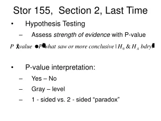
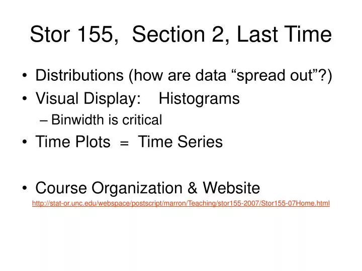
Stor 155, Section 2, Last Time. Distributions (how are data “spread out�) Visual Display: Histograms Binwidth is critical Time Plots = Time Series Course Organization & Website http://stat-or.unc.edu/webspace/postscript/marron/Teaching/stor155-2007/Stor155-07Home.html.

E N D
Stor 155, Section 2, Last Time • Distributions (how are data “spread out”?) • Visual Display: Histograms • Binwidth is critical • Time Plots = Time Series • Course Organization & Website http://stat-or.unc.edu/webspace/postscript/marron/Teaching/stor155-2007/Stor155-07Home.html
Reading In Textbook Approximate Reading for Today’s Material: Pages 40-55 Approximate Reading for Next Class: Pages 64-83
And now for something completely different Is this class too “monotone”? • Easier to understand? • Calm environment enhances learning? • Or does it induce somnolence? What is “somnolence”? Google definition: Sleepiness, a condition of semiconsciousness approaching coma.
And now for something completely different An experiment: • Pull out any coins you have with you • How many of you have: • >= 1 penny? • >= 1 nickel? • >= 1 dime? • >= 1 quarter? • Choose most frequent denomination
And now for something completely different Collect data (into Spreadsheet): • Years stamped on coins (chosen denomination) • Many as person has • Enter into spreadsheet • Look at “distribution” using histogram
And now for something completely different • Predicted Answer • From Text Book, Problem 1.32 • Distribution is Left Skewed • Works out as predicted? • Why? • Note: most skewed dist’ns seem to be: Right Skewed
Exploratory Data Analysis 4 Numerical Summaries of Quant. Variables: Idea: Summarize distributional information (“center”, “spread”, “skewed”) In Text, Sec. 1.2 for data (subscripts allow “indexing numbers” in list)
Numerical Summaries • “Centers” (note there are several) • “Mean” = Average = • Greek letter “Sigma”, for “sum” In EXCEL, use “AVERAGE” function
Numerical Summaries of Center • “Median” = Value in middle (of sorted list) Unsorted E.g: Sorted E.g: 3 0 1 1 27 “in middle”? (no) 2 better “middle”! 2 3 0 27 EXCEL: use function “MEDIAN”
Difference Betw’n Mean & Median Symmetric Distribution: Essentially no difference Right Skewed Distribution: 50% area 50% area M bigger since “feels tails more strongly”
Difference Betw’n Mean & Median Outliers (unusual values): Simple Web Example: http://www.stat.sc.edu/~west/applets/box.html • Mean feels outliers much more strongly • Leaves “range of most of data” • Good notion of “center”? (perhaps not) • Median affected very minimally • Robustness Terminology: Median is “resistant to the effect of outliers”
Difference Betw’n Mean & Median A richer web example: Publisher’s Web Site: Statistical Applets: Mean & Median • For Symmetric distributions: • Both are same • Add an outlier: • Mean feels it much more strongly • Implication for “bad data”: can be very bad • Two Clusters: • Median jumps more quickly • Mean more stable (better?)
Computation using Excel Some Toy Examples: http://stat-or.unc.edu/webspace/postscript/marron/Teaching/stor155-2007/Stor155Eg3Done.xls • Compute Using Excel Functions • Mean feels location of data on number line • Median feels location of data in sorted list • Median breaks tie by averaging center points
Numerical Centerpoint HW HW: 1.46 a, 1.47, 1.49 • Use EXCEL
And now for something completely different Check out this small quick movie clip:
And now for something completely different Suggestions for other things to show here are very welcome…. • Movie Clips… • Music… • Jokes… • Cartoons… • …
Numerical Summaries (cont.) • “Spreads” (again there are several) 1. Range = biggest - smallest range Problems: • Feels only “outliers” • Not “bulk of data” • Very non-resistant to outliers
Numerical Summaries of Spread • Variance = = “average squared distance to “ EXCEL: VAR Drawback: units are wrong e. g. For in feet is in square feet
Numerical Summaries of Spread • Standard Deviation EXCEL: STDEV • Scale is right • But not resistant to outliers • Will use quite a lot later (for reasons described later)
Interactive View of S. D. Interesting web example (manipulate histogram): http://www.ruf.rice.edu/~lane/stat_sim/descriptive/index.html • Note SD range centered at mean • Can put SD “right near middle” (densely packed data) • Can put SD at “edges of data” (U shaped data) • Can put SD “outside of data” (big spike + outlier) • But generally “sensible measure of spread”
Variance – S. D. HW C3: For the data set in 1.46 (i.e. 1.37), find the: • Variance (1620) • Standard Deviation (40.2) • Use EXCEL
Numerical Summaries of Spread • Interquartile Range = IQR Based on “quartiles”, Q1 and Q3 (idea: shows where are 25% & 75% “through the data”) 25% 25% 25% 25% Q1 Q2 = median Q3 IQR = Q3 – Q1
Quartiles Example Revisit Hidalgo Stamp Thickness example: http://stat-or.unc.edu/webspace/postscript/marron/Teaching/stor155-2007/Stor155Eg6Done.xls Right skewness gives: • Median < Mean (mean “feels farther points more strongly”) • Q1 near median • Q3 quite far (makes sense from histogram)
Quartiles Example A look under the hood: http://stat-or.unc.edu/webspace/postscript/marron/Teaching/stor155-2007/Stor155Eg6Raw.xls • Can compute as separate functions for each • Or use: Tools Data Analysis Descriptive Stats • Which gives many other measures as well • Use “k-th largest & smallest” to get quartiles
5 Number Summary • Minimum • Q1 - 1st Quartile • Median • Q3 - 3rd Quartile • Maximum Summarize Information About: • Center - from 3 • Spread - from 2 & 4 (maybe 1 & 5) • Skewness - from 2, 3 & 4 • Outliers - from 1 & 5
5 Number Summary How to Compute? http://stat-or.unc.edu/webspace/postscript/marron/Teaching/stor155-2007/Stor155Eg6Done.xls • EXCEL function QUARTILE • “One stop shopping” • IQR seems to need explicit calculation
Rule for Defining “Outliers” Caution: There are many of these Textbook version: Above Q3 + 1.5 * IQR Below Q1 – 1.5 * IQR For stamps data: http://stat-or.unc.edu/webspace/postscript/marron/Teaching/stor155-2007/Stor155Eg6Done.xls • No outliers at “low end” • Some at “high end”
Box Plot • Additional Visual Display Device • Again legacy from pencil & paper days • Not supported in EXCEL • So we won’t do • Main use: comparing populations • Example: Figure from text
Box Plot • Main use: comparing populations • Example: Figure from text • Want to do this? Find better software package than Excel
And now for something completely different Recall Distribution of majors of students in this course:
And now for something completely different How about a business manager joke? How many managers does it take to replace a light bulb?
And now for something completely different How about a business manager joke? How many managers does it take to replace a light bulb? Two. One to find out if it needs changing, and one to tell an employee to change it. Source: http://www.joblatino.com/jokes/managers.html
Linear Transformations Idea: What happens to data & summaries, when data are: “shifted and scaled” i.e. “panned and zoomed” Math: Scaled by a Shifted by b
Linear Transformations Effect on linear summaries: • Centerpoints, and “follow data”: . • Spreads, and “feel scale, not shift”: .
Most Useful Linear Transfo. “Standardization” Goal: put data sets on “common scale” Approach: • Subtract Mean , to “center at 0” • Divide by S.D. , to “give common SD = 1”
Standardization Result is called “z-score”: Note that Thus is interpreted as: “number of SDs from the mean”
Standardization Example Next time: work in Excel command: STANDARDIZE
Standardization Example Buffalo Snowfall Data: http://stat-or.unc.edu/webspace/postscript/marron/Teaching/stor155-2007/Stor155Eg7Done.xls • Standardized data have same (EXCEL default) histogram shape as raw data. (Since axes and bin edges just follow the transformation) • i.e. “shape” doesn’t depend on “scaling”
Standardization Example A look under the hood: http://stat-or.unc.edu/webspace/postscript/marron/Teaching/stor155-2007/Stor155Eg7Raw.xls Compute AVERAGE and SD • Standardize by: • Create Formula in cell B2 • Drag downwards • Keep Mean and SD cells fixed using $s 3. Check stand’d data have mean 0 & SD 1 note that “8.247E-16 = 0”
Standardization HW C4: For data in 1.17, use EXCEL to: a. Give the list of standardized scores b. Give the Z-score for: (i) the mean (0) (ii) the median (-0.223) (iii) the smallest (-1.21) (iv) the largest (2.77) 1.59a, 1.73