Download

1 / 102
1.03k likes | 1.51k Vues
Approximate Nearest Neighbor - Applications to Vision & Matching. Lior Shoval Rafi Haddad. Approximate Nearest Neighbor Applications to Vision & Matching. Object matching in 3D Recognizing cars in cluttered scanned images A. Frome, D. Huber, R. Kolluri, T. Bulow, and J. Malik

E N D
Approximate Nearest Neighbor - Applications to Vision & Matching Lior Shoval Rafi Haddad
Approximate Nearest NeighborApplications to Vision & Matching • Object matching in 3D • Recognizing cars in cluttered scanned images • A. Frome, D. Huber, R. Kolluri, T. Bulow, and J. Malik • Video Google • A Text Retrieval Approach to object Matching in Videos • Sivic, J. and Zisserman, A
Object Matching • Input: • An object and a dataset of models • Output: • The most “similar” model • Two methods will be presented • Voting based method • Cost based method Model Sn Model S1 Model S2 Object Sq …
A descriptor based Object matching - Voting • Every descriptor vote for the model that gave the closet descriptor • Choose the model with the most votes • Problem • The hard vote discards the relative distances between descriptors Model Sn Model S1 Model S2 Object Sq …
A descriptor based Object matching - Cost • Compare all object descriptors to all target model descriptors Model Sn Model S1 Model S2 Object Sq …
Matching - Nearest Neighbor • In order to match the object to the right model a NN algorithm is implemented • Every descriptor in the object is compared to all descriptors in the model • The operational cost is very high.
Matching - Nearest Neighbor • E.g: • Q – 160 descriptors in the object • N – 83,640 [ref. desc.] X 12 [rotations] ~ 1E6 descriptors in the models • Exact NN - takes 7.4 Sec on 2.2GHz processor per one object descriptor
Speeding search with LSH • Fast search techniques such as LSH (Locality-sensitive hashing) can reduce the search space by order of magnitude • Tradeoff between speed and accuracy • LSH – Dividing the high dimensional feature space into hypercubes, devided by a set of k randomly-chosen axis parallel hyperplanes & l different sets of hypercubes
LSH - Results • Taking the best 80/160 descriptors • Achieving close results with fewer descriptors
Descriptor based Object matching – Reducing Complexity • Approximate nearest neighbor • Dividing the problem to two stages • Preprocessing • Querying • Locality-Sensitive Hashing (LSH) • Or...
Video Google • A Text Retrieval Approach to object Matching in Videos
Query Results
Interesting facts on Google The most used search engine in the web
How many pages Google search? a. Around half a billion b. Around 4 billions c. Around 10 billions d. Around 50 billions
How many machines do Google use? a. 10 b. Few hundreds c. Few thousands d. Around a million
Video Google: On-line Demo Samples Run Lola Run: Supermarket logo (Bolle)Frame/shot 72325 / 824 Red cube logo:Entry frame/shot 15626 / 174 Rolette #20 Frame/shot94951 / 988 Groundhog Day: Bill Murray's tiesFrame/shot 53001/294Frame/shot 40576/208 Phil's home:Entry frame/shot 34726/172
Video Google • Text Google • Analogy from text to video • Video Google processes • Experimental results • Summary and analysis
Text retrieval overview • Word & Document • Vocabulary • Weighting • Inverted file • Ranking
Words & Documents • Documents are parsed into words • Common words are ignored (the, an, etc) • This is called ‘stop list’ • Words are represented by their stems • ‘walk’, ‘walking’, ‘walks’’walk’ • Each word is assigned a unique identifier • A document is represented by a vector • With components given by the frequency of occurrence of the words it contains
Vocabulary • The vocabulary contains K words • Each document is represented by a K components vector of words frequencies (0,0, … 3,… 4,…. 5, 0,0)
Example: “…… Representation, detection and learning are the main issues that need to be tackled in designing a visual system for recognizing object. categories …….”
Parse and clean represent detect learn Representation, detection and learning are the main issue tackle design main issues that need to be tackled in designing visual system recognize category a visual system for recognizing object categories. …
Creating document vector ID • Assign unique id to each word • Create a document vector of size K with word frequency: • (3,7,2,………)/789 • Or compactly with the original order and position
Weighting • The vector components are weighted in various ways: • Naive - Frequency of each word. • Binary– 1 if word appear 0 if not. • tf-idf - ‘Term Frequency – Inverse Document Frequency’
tf-idf Weighting - Number of occurrences of word i in document - Total number of words in the document - The number of documents in the whole database - The number of occurrences of term i in the whole database => “Word frequency” X “Inverse document frequency” => All documents are equal!
Inverted File – Index • Crawling stage • Parsing all documents to create document representing vectors • Creating word Indices • An entry for each word in the corpus followed by a list of all documents (and positions in it)
Querying • Parsing the query to create query vectorQuery: “Representation learning” Query Doc ID = (1,0,1,0,0,…) • Retrieve all documents ID containing one of the Query words ID (Using the invert file index) • Calculate the distance between the query and document vectors (angle between vectors) • Rank the results
Ranking the query results • Page Rank (PR) • Assume page A has page T1,T2…Tn links to it • Define C(X) as the number of links in page X • d is a weighting factor ( 0≤d≤1) • Word Order • Font size, font type and more
Corpus Film The Visual Analogy ??? Word Stem ??? Document Frame Text Visual
Detecting “Visual Words” • “Visual word” Descriptor • What is a good descriptor? • Invariant to different view points, scale, illumination, shift and transformation • Local Versus Global • How to build such a descriptor ? • Finding invariant regions in the frame • Representation by a descriptor
Finding invariant regions • Two types of ‘viewpoint covariant regions’, are computed for each frame • SA – Shape Adapted • MS - Maximally Stable
SA – Shape Adapted • Finding interest point using Harris corner detector • Iteratively determining the ellipse center, scale and shape around the interest point • Reference - Baumberg
MS - Maximally Stable • Intensity water shade image segmentation • Iteratively determining the ellipse center, scale and shape • Reference - Matas
Why two types of detectors ? • They are complementary representation of a frame • SA regions tends to centered at corner like features • MS regions correspond to blobs of high contrast (such as dark window on a gray wall) • Each detector describes a different “vocabulary” (e.g. the building design and the building specification)
MS - MA example MS – yellow SA - cyan Zoom